3 Model Free Policy Control

Model-free policy evaluation(control)은 다음의 상황에서 유용하다.

1. MDP 모델이 안알려졌지만, MDP로부터 trajectory sampling이 되는 경우
2. MDP 모델은 알려졌으나, value function 계산이 infeasible한 경우

5.1 Generalized Policy Iteration

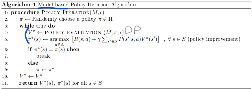
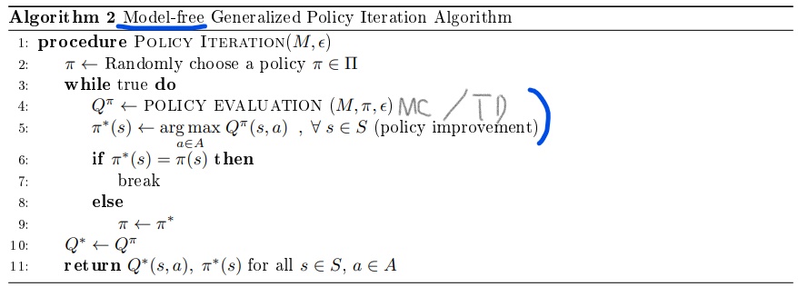
Model-based는 직접적으로 policy를 업데이트하는 꼴이고 Model-free는 Q-function에 기반해서 업데이트한다.

Model-free의 경우 주의할 점은 policy $\pi$는 어떤 action이든 선택할 확률이 있긴 해야 $Q^\pi(s,a)$를 정의할 수 있다.

5.2 Importance of Exploration

5.2.1 Exploration

Policy $\pi$는 어디든 갈 확률이 있어야 Q-value를 구할 수 있다.

5.2.2 $\epsilon$-greedy policy

현재의 Q-value estimate에 대해 exploration(suboptimal)과 exploitation(greedy) 사이를 조절해야한다.

가장 단순한 방법은 random action을 취할 확률 $\epsilon$과 greedy action을 취할 확률 $1-\epsilon$을 주는 것이다.

$$\pi(a \mid s)=\left\{\begin{array}{ll} a & \text { with probability } \frac{\epsilon}{|A|} \\ \arg \max _{a} Q^{\pi}(s, a) & \text { with probability } 1-\epsilon \end{array}\right.$$

5.2.3 Monotonic $\epsilon$-greedy Policy Improvement

Theorem 5.1 (Monotonic $\epsilon$-greedy Policy Improvement)

​ Let $\pi_i$ be an $\epsilon$-greedy policy.

​ Let $\pi_{i+1}$ be the $\epsilon$-greedy policy w.r.t. $Q^{\pi_i}$

​ $\pi_{i+1}$ is a monotonic improvement on policy $\pi_i$; $V^{\pi_{i+1}} \geq V^{\pi_{i}}$

(증명)

$$\begin{aligned} Q^{\pi_{i}}\left(s, \pi_{i+1}(s)\right) &=\sum_{a \in A} \pi_{i+1}(a \mid s) Q^{\pi_{i}}(s, a) \\ &=\frac{\epsilon}{|A|} \sum_{a \in A} Q^{\pi_{i}}(s, a)+(1-\epsilon) \max _{a^{\prime}} Q^{\pi_{i}}\left(s, a^{\prime}\right) \\ &=\frac{\epsilon}{|A|} \sum_{a \in A} Q^{\pi_{i}}(s, a)+(1-\epsilon) \max _{a^{\prime}} Q^{\pi_{i}}\left(s, a^{\prime}\right) \frac{1-\epsilon}{1-\epsilon} \\ &=\frac{\epsilon}{|A|} \sum_{a \in A} Q^{\pi_{i}}(s, a)+(1-\epsilon) \max _{a^{\prime}} Q^{\pi_{i}}\left(s, a^{\prime}\right) \sum_{a \in A} \frac{\pi_{i}(a \mid s)-\frac{\epsilon}{|A|}}{1-\epsilon} \\ &=\frac{\epsilon}{|A|} \sum_{a \in A} Q^{\pi_{i}}(s, a)+(1-\epsilon) \sum_{a \in A} \frac{\pi_{i}(a \mid s)-\frac{\epsilon}{|A|}}{1-\epsilon} \max _{a^{\prime}} Q^{\pi_{i}}\left(s, a^{\prime}\right) \\ & \geq \frac{\epsilon}{|A|} \sum_{a \in A} Q^{\pi_{i}}(s, a)+(1-\epsilon) \sum_{a \in A} \frac{\pi_{i}(a \mid s)-\frac{\epsilon}{|A|}}{1-\epsilon} Q^{\pi_{i}}(s, a) \\ &=\sum_{a \in A} \pi_{i}(a \mid s) Q^{\pi_{i}}(s, a) \\ &=V^{\pi_{i}}(s) \end{aligned}$$

​ 그리고, policy improvement theorem이 말하길 $Q^{\pi_{i}}\left(s, \pi_{i+1}(s)\right) \geq V^{\pi_{i}}(s)$는 $V^{\pi_{i+1}}(s) \geq V^{\pi_{i}}(s)$를 의미한다.

5.2.3 Greedy in the limit of exploration

Convergence를 보장하기 위해 naive한 $\epsilon$-greedy policy를 좀 더 정제해보자.

Definition 5.1 (Greedy in the Limit of Infinite Exploration (GLIE)).

​ Policy $\pi$ is GLIE if

1. All state-action pairs are visited an infinite times;

   즉, $i$번째 episode까지의 $(s,a)$ 방문수를 $N_i(s,a)$라고 하면, $\lim _{i \rightarrow \infty} N_{i}(s, a) \rightarrow \infty$

2. The behavior policy converges to the greedy policy w.r.t. the learned Q-function $q(s,a)$;
   $\lim _{i \rightarrow \infty} \pi_{i}(a \mid s)=\arg \max _{a} q(s, a) \text { with probability } 1$

---

GLIE를 만족하는 greedy policy의 대표적인 예시는 $\epsilon_i = \frac{1}{i}$로 두는 것이다.

5.3 Monte Carlo Control

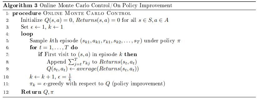
Theorem 5.2

​ 알고리즘 3의 $\epsilon$-greedy policy가 GLIE면 optimal Q-function으로 수렴이 보장된다. $Q(s, a) \rightarrow q(s, a)$

5.4 Temporal Difference Methods for Control

TD-style model-free control은 on-policy와 off-policy가 있다.

SARSA는 Q-value를 update하는데 $(s,a,r, s’, a’)$을 사용한다.

이는 on-policy 알고리즘으로 $s\rightarrow a$와 $s’\rightarrow a’$이 똑같은 policy를 따른다.

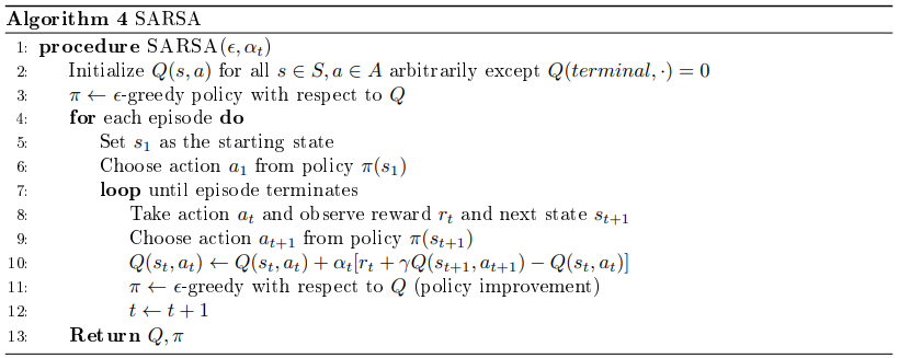
MC처럼 SARSA의 수렴은 extra condition에 의해 만족될 수 있다.

Theorem 5.3

​ SARSA for finite-state and finite-action MDP converges to optimal action-value $Q(s, a) \rightarrow q(s, a)$ if

1. The sequence of policies $\pi$ is GLIE
2. Step-size $\alpha_t$ satisfies Robin-Munro sequence $\begin{array}{l}
   \sum_{t=1}^{\infty} \alpha_{t}=\infty \\
   \sum_{t=1}^{\infty} \alpha_{t}^{2}<\infty
   \end{array}$

5.5 Importance sampling for off-policy TD

TD policy evaluation은 $V(s) \leftarrow V(s)+\alpha\left(r+\gamma V\left(s^{\prime}\right)-V(s)\right)$으로 이뤄진다.

만약 estimate policy $\pi_e$와 behavior policy $\pi_b$가 다른 경우,

$$V^{\pi_{e}}(s) \rightarrow V^{\pi_{e}}(s)+\alpha\left[\frac{\pi_{e}(a \mid s)}{\pi_{b}(a \mid s)}\left(r+\gamma V^{\pi_{e}}\left(s^{\prime}\right)-V^{\pi_{e}}(s)\right)\right]$$

MC method로 이를 하려면 importance weight을 history의 길이만큼 곱해야 때문에 분산이 크다.

TD method의 경우 one step이라 importance weight을 한번만 곱해서 구하고 분산이 작다.

5.6 Q-learning

SARSA가 $s \rightarrow a$와 $s’\rightarrow a’$의 policy가 같다는 sense에서 on-policy라고 하였다.

이게 다르다는 sense에서 off-policy 알고리즘인 Q-learning을 소개하겠다.

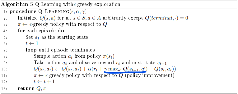
이는 TD error $r_{t}+\gamma Q\left(s_{t+1}, a_{t+1}\right)$을 $r_{t}+\gamma \max _{a^{\prime}} Q\left(s_{t+1}, a^{\prime}\right)$로 대체한 것이다.

next state $s’$에서, 현재 policy에 기반해서 next action $a’$이 나오는 게 아니라 현재 $Q$에 maximization으로 나온다.

6 Maximization Bias

6.1 Examples: Coins

두개의 identical fair coin이 있는데 아무것도 모르는 상황이다.

앞면이면 +1 뒷면이면 -1의 reward가 발생한다고 하자.

Q1. 어떤 코인이 돈을 더 벌어다줄까?

Q2. Q1에서 말한 코인은 얼마나 줄까?

이 질문에 대한 답을 위해 두개의 동전을 던지고 잘나온 동전을 골라서 답을 한다면 Q2에 대한 답은 $\frac{3}{4} \times(1)+\frac{1}{4} \times(-1)=0.5$이다.

---

이런 문제는 두 선택지 중에 결과가 더 나은걸 골라서 estimate하는 경우에 발생한다.

이를 피하기 위해선 더 나은 코인을 선택한 다음에 한번 더 던져서 Q2를 답해야 한다.

6.2 Maximization Bias in Reinforcement Learning

Coins의 예시에 맞춰서 One-step MDP with $\left\{\begin{array}{l}
\text{two actions } a_1, a_2\\
R(s, a_1) = R(s, a_2)=0
\end{array}\right.$을 고려해보자.

이 경우엔, $Q(s, a_1) = Q(s, a_2) = V(s) = 0$이다.

샘플링을 통해 Q에 대한 estimator를 $\hat Q (s, a_1), \hat Q(s, a_2)$라고 하자. 이들은 unbiased estimator이다.

Let $\hat \pi = \arg \max _a \hat Q(s, a)$. Then,

$$\begin{aligned} \hat{V}(s) &=E\left[\max \left(\hat{Q}\left(s, a_{1}\right), \hat{Q}\left(s, a_{2}\right)\right]\right.\\ & \geq \max \left(E\left[\hat{Q}\left(s, a_{1}\right)\right], E\left[\hat{Q}\left(s, a_{2}\right)\right]\right) \\ &=\max (0,0) \\ &=0=V^{*}(s) \end{aligned}$$

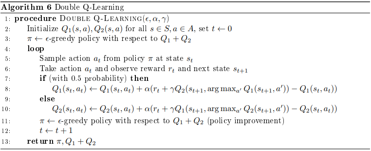
6.3 Double Q-Learning

max와 estimate을 구분해놓음으로 bias를 제거할 수 있다.

Double Q-Learning의 핵심은 $Q_1$과 $Q_2$중에 랜덤하게 하나는 max에 사용하고 하나는 estimate에 사용하는 것이다.