0. Abstract

Monotonic improvement가 보장된 policy gradient 알고리즘을 설명하겠다.

비록 이론적 결과에 대한 approximation을 하게 되지만 여전히 monotonic improvement를 주는 경향이 있다.

1. Introduction

이론적 결과로 특정한 surrogate objective function을 최적화한다면 policy improvement가 보장됨을 보이겠다. (Algorithm 1)

그 다음, 실용성을 위해 이에 대한 근사인 TRPO를 소개하도록 하겠다.

TRPO에 2가지 버전 single-path와 vine이 있는데 후자는 simulation에서만 가능하다.

실험적으로, TRPO가 Atari, swimming, walking 등에서 complex policy를 학습할 수 있음을 보이겠다.

2. Preliminaries

Infinite-horizon discounted Markov decision process (MDP) $\left(\mathcal{S}, \mathcal{A}, P, r, \rho_{0}, \gamma\right)$

$\mathcal S$ is a finite set of states
$\mathcal A$ is a finite set of actions
$P: \mathcal{S} \times \mathcal{A} \times \mathcal{S} \rightarrow \mathbb{R}$ is the transition probability distribution
$r: \mathcal{S} \rightarrow \mathbb{R}$ is the reward function
$\rho_{0}: \mathcal{S} \rightarrow \mathbb{R}$ is the distribution of the initial state $s_0$
$\gamma \in(0,1)$ is the discount factor

Let

$\pi: \mathcal{S} \times \mathcal{A} \rightarrow[0,1]$ is a stochastic policy
$\eta(\pi)=\mathbb{E}_{s_{0}, a_{0}, \ldots}\left[\sum_{t=0}^{\infty} \gamma^{t} r\left(s_{t}\right)\right]$ is the expected discounted reward
- $s_{0} \sim \rho_{0}\left(s_{0}\right)$
- $a_{t} \sim \pi\left(a_{t} \mid s_{t}\right)$
- $s_{t+1} \sim P\left(s_{t+1} \mid s_{t}, a_{t}\right)$
$Q_{\pi}\left(s_{t}, a_{t}\right)=\mathbb{E}_{s_{t+1}, a_{t+1}, \ldots}\left[\sum_{l=0}^{\infty} \gamma^{l} r\left(s_{t+l}\right)\right]$ is the state-action value function
$V_{\pi}\left(s_{t}\right)=\mathbb{E}_{a_{t}, s_{t+1}, \ldots}\left[\sum_{l=0}^{\infty} \gamma^{l} r\left(s_{t+l}\right)\right]$ is the state value function
$A_{\pi}(s, a)=Q_{\pi}(s, a)-V_{\pi}(s)$ is the advantage function

Kakede & Langford (2002)에 대한 요약

$\begin{aligned} \eta(\tilde{\pi}) &=\eta(\pi)+\mathbb{E}_{s_{0}, a_{0}, \cdots \sim \tilde{\pi}}\left[\sum_{t=0}^{\infty} \gamma^{t} A_{\pi}\left(s_{t}, a_{t}\right)\right] \\ &=\eta(\pi)+\sum_{s} \rho_{\tilde{\pi}}(s) \sum_{a} \tilde{\pi}(a \mid s) A_{\pi}(s, a) \end{aligned}$

where $\rho_{\pi}(s)=P\left(s_{0}=s\right)+\gamma P\left(s_{1}=s\right)+\gamma^{2} P\left(s_{2}=s\right)+\ldots$

직감적으로, $\tilde \pi$에 대한 evaluation을 $\pi$를 가지고 할 수 있다는 것이다.
만약 모든 state $s$에 대해서, $\sum_{a} \tilde{\pi}(a \mid s) A_{\pi}(s, a) \geq 0$ 일 경우 policy improvement가 보장된다.

하지만, 실제로는 $A_{\pi}(s, a)$는 샘플링 기반으로 approximation하게 될 것이다.

그 때, trajectory sample은 old policy $\pi$에서 뽑은 것을 사용할 것이다.

그 경우엔 $\rho_{\tilde{\pi}}(s)$는 장애물이 될 것이다.

이를 대처하기 위해 local approximation을 도입한다.

$L_{\pi}(\tilde{\pi})=\eta(\pi)+\sum_{s} \rho_{\pi}(s) \sum_{a} \tilde{\pi}(a \mid s) A_{\pi}(s, a)$

이는 굉장히 좋은 근사이다.

$L_{\pi_{\theta_{0}}}\left(\pi_{\theta_{0}}\right)=\eta\left(\pi_{\theta_{0}}\right)$
$\left.\nabla_{\theta} L_{\pi_{\theta_{0}}}\left(\pi_{\theta}\right)\right|_{\theta=\theta_{0}}=\left.\nabla_{\theta} \eta\left(\pi_{\theta}\right)\right|_{\theta=\theta_{0}} \quad \because$ Sutton, 1999

결론은, 작은 step만큼 policy update할 경우 $L$의 증가가 곧 $\eta$의 증가를 의미한다.

하지만 충분히 작은 step에 대한 애매모호함이 있기에 이들은 conservative policy iteration을 도입하였다.

Let $\pi^{\prime}=\arg \max _{\pi^{\prime}} L_{\pi_{\mathrm{old}}}\left(\pi^{\prime}\right)$
Let $\pi_{\text {new }}(a \mid s)=(1-\alpha) \pi_{\text {old }}(a \mid s)+\alpha \pi^{\prime}(a \mid s)$
Then, $\eta\left(\pi_{\text {new }}\right) \geq L_{\pi_{\text {old }}}\left(\pi_{\text {new }}\right)-\frac{2 \epsilon \gamma}{(1-\gamma)^{2}} \alpha^{2}$ where $\epsilon=\max _{s}\left|\mathbb{E}_{a \sim \pi^{\prime}(a \mid s)}\left[A_{\pi}(s, a)\right]\right|$

하지만 이 lower bound는 mixture policy에서 적용되기 때문에 일반적이지 못하다.

3. Monotonic Improvement Guarantee for General Stochastic Policies

Let

$D_{T V}(p | q)=\frac{1}{2} \sum_{i}\left|p_{i}-q_{i}\right|$
$D_{\mathrm{TV}}^{\max }(\pi, \tilde{\pi})=\max _{s} D_{T V}(\pi(\cdot \mid s) | \tilde{\pi}(\cdot \mid s))$

Theorem 1

Let $\alpha=D_{\mathrm{TV}}^{\max }\left(\pi_{\mathrm{old}}, \pi_{\mathrm{new}}\right)$. Then,

$\begin{aligned} \eta\left(\pi_{\text {new}}\right) &\geq L_{\pi_{\text {old}}}\left(\pi_{\text {new }}\right)-\frac{4 \epsilon \gamma}{(1-\gamma)^{2}} \alpha^{2} \quad \text{where } \epsilon=\max _{s, a}\left|A_{\pi}(s, a)\right| \\ &\geq L_{\pi_{\text{old }}}(\pi_{\text{new }})-\frac{4 \epsilon \gamma}{(1-\gamma)^{2}} D_{\mathrm{KL}}^{\max }(\pi_{\text{old }}, {\pi_{\text{new }}}) \quad \quad \because D_{T V}(p \| q)^{2} \leq D_{\mathrm{KL}}(p \| q) \end{aligned}$

위의 정리에 기반하여 monotonic increasing policy iteration algorithm을 제안한다.

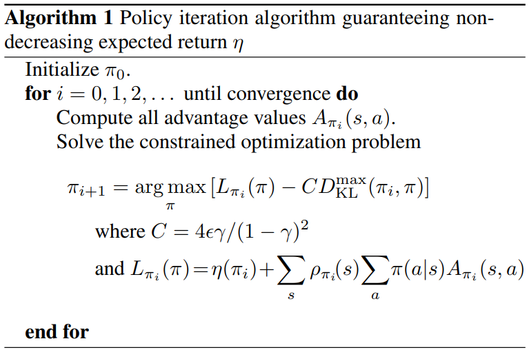
이 알고리즘은 $A_{\pi}$에 대한 evaluation이 가능하다고 암묵적으로 가정한다.

그 상황에서 monotonically improving sequence of policies가 생성된다.

Let $M_i(\pi) = L_{\pi_i}(\pi_{i+1}) - C D_{\mathrm{KL}}^{\max }\left(\pi_{i}, \pi\right)$.

Since $\eta\left(\pi_{i+1}\right) \geq M_{i}\left(\pi_{i+1}\right) \quad$ and $ \quad \eta\left(\pi_{i}\right)=M_{i}\left(\pi_{i}\right)$,

$\eta\left(\pi_{i+1}\right)-\eta\left(\pi_{i}\right) \geq M_{i}\left(\pi_{i+1}\right)-M\left(\pi_{i}\right) \geq 0$

TRPO는 알고리즘 1에 대한 근사이다.

Large update를 robust하게 허용하기 위해 페널티 텀 $C D_{\mathrm{KL}}^{\max }\left(\pi_{i}, \pi\right)$을 없애고 constraint를 건다.

4. Optimization of Parameterized Policies

이론적인 알고리즘 1은 $A_{\pi}$에 대한 evaluation이 가능함을 가정하였고 policy search $\pi_{i+1}=\underset{\pi}{\arg \max }\left[…\right]$의 computational complexity를 고려하지 않았다.

이번 장과 다음 장에서 finite sample과 parameter로 구현되는 practical algorithm을 도출하겠다.

Let

$\eta(\theta):=\eta\left(\pi_{\theta}\right)$
$L_{\theta}(\tilde{\theta}):=L_{\pi_{\theta}}\left(\pi_{\tilde{\theta}}\right)$
$D_{\mathrm{KL}}(\theta | \tilde{\theta}):=D_{\mathrm{KL}}\left(\pi_{\theta} | \pi_{\tilde{\theta}}\right)$

Then, $\pi_{i+1}=\underset{\pi}{\arg \max }\left[L_{\pi_{i}}(\pi)-C D_{\mathrm{KL}}^{\max }\left(\pi_{i}, \pi\right)\right]$ is expressed as

$\underset{\theta}{\operatorname{maximize}}\left[L_{\theta_{\text {old }}}(\theta)-C D_{\mathrm{KL}}^{\max }\left(\theta_{\text {old }}, \theta\right)\right]$

페널티 텀을 집어 넣는 방식의 경우 step size가 정말 작을 수도 있다.

Robust한 방식으로 large step을 취하기 위해서, trust region constraint를 채택하자.

$\underset{\theta}{\operatorname{maximize}} L_{\theta_{\text {old }}}(\theta) \quad \text { subject to } D_{\mathrm{KL}}^{\max }\left(\theta_{\mathrm{old}}, \theta\right) \leq \delta$

$\delta$를 허용된 step size라고 해석하면 된다.

$D_{\mathrm{KL}}^{\max }\left(\theta_{\mathrm{old}}, \theta\right) \leq \delta$를 확인하기 위해서 모든 state에 대해 KL-divergence를 구하는 것은 비실용적이다.

Approximation (sampling 기반)으로 constraint를 확인하기 위해 average KLD로 바꾸자.

$\underset{\theta}{\operatorname{maximize}} L_{\theta_{\text {old }}}(\theta) \quad \text { subject to } \overline{D}_{\mathrm{KL}}^{\rho_{\theta_{\mathrm{old}}}}\left(\theta_{\mathrm{old}}, \theta\right) \leq \delta$

실험적으로 이러한 constraint의 변경은 큰 성능차이를 불러일으키지 않음을 확인하였다.

5. Sample-Based Estimation of the Objective and Constraint

4장에서 정의한 objective function과 constraint function을

$\underset{\theta}{\operatorname{maximize}} \sum_{s} \rho_{\theta_{\text {old }}}(s) \sum_{a} \pi_{\theta}(a \mid s) A_{\theta_{\text {old }}}(s, a) \quad \text { subject to } \overline{D}_{\mathrm{KL}}^{\rho_{\theta_{\mathrm{old}}}}\left(\theta_{\mathrm{old}}, \theta\right) \leq \delta$

approximation하는 방법을 소개한다.

$\sum_{s} \rho_{\theta_{\text {old }}}(s)[\ldots] \quad \Longrightarrow \quad \frac{1}{1-\gamma} \mathbb{E}_{s \sim \rho_{\theta_{\text {old }}}}[\ldots]$ ;
$A_{\theta_{\mathrm{old}}} \quad \Longrightarrow \quad Q_{\theta_{\text {old }}}$ ;
$\sum_{a} \pi_{\theta}\left(a \mid s_{n}\right) A_{\theta_{\text {old }}}\left(s_{n}, a\right)=\mathbb{E}_{a \sim q}\left[\frac{\pi_{\theta}\left(a \mid s_{n}\right)}{q\left(a \mid s_{n}\right)} A_{\theta_{\text {old }}}\left(s_{n}, a\right)\right]$

위의 세가지 사실들은 1. normalize; 2. $V$텀은 $\theta$에 독립적임; 3. policy $\pi_{old}$에서 뽑은 샘플로 MC approximation을 하기 위해 importance samling 도입한 것이다.

위의 세가지 사실을 활용하면 optimization 식을 다르게 표현할 수 있다.

$\underset{\theta}{\operatorname{maximize}} \mathbb{E}_{s \sim \rho_{\theta_{\text {old }}}, a \sim q}\left[\frac{\pi_{\theta}(a \mid s)}{q(a \mid s)} Q_{\theta_{\text {old }}}(s, a)\right] \quad \text { subject to } \mathbb{E}_{s \sim \rho_{\theta_{\text {old }}}}\left[D_{\mathrm{KL}}\left(\pi_{\theta_{\text {old }}}(\cdot \mid s) \| \pi_{\theta}(\cdot \mid s)\right)\right] \leq \delta$

이제 objective function과 constraint function을 estimate하는 두가지 방법을 소개하겠다.

5.1 Single path

Individualized trajectories sampling에 기반한 방식이다.

이는 policy gradient estimation에서 일반적으로 사용된다.

Sample $s_0 \sim \rho_0$
Simulate one trajectory $a_{0}, s_{1}, a_{1}, \ldots, s_{T-1}, a_{T-1}, s_{T} \sim\pi_{\theta_{\text{old}}} \times P$
MC approximation

5.2 Vine

Sample $s_0 \sim \rho_0$
Simulate multiple trajectories $a_{0}, s_{1}, a_{1}, \ldots, s_{T-1}, a_{T-1}, s_{T} \sim\pi_{\theta_{\text{old}}} \times P$
Choose $N$ states along these trajectories; $\{ s_{1}, s_{2}, \ldots, s_{N}\}$, called rollout set
For each state $s_n$ in the rollout set, sample $K$ actions; $a_{n, k} \sim q\left(\cdot \mid s_{n}\right)$ s.t.
- $ \text{supp}(\pi_{\text{old}}(\cdot \mid s_n)) \subseteq \text{supp}(q(\cdot \mid s_n))$
- continuous action을 다룰 땐, $q\left(\cdot \mid s_{n}\right)=\pi_{\theta_{\text{old}}}\left(\cdot \mid s_{n}\right)$이 좋고
- discrete action을 다룰 땐, $q\left(\cdot \mid s_{n}\right) = \text{Uni}$가 좋다. (exploration 측면에서)
…

모르겠다.

Vine은 single path method보다 분산이 낮아서 좋다.

하지만 simulation 밖에서는 안되는 방법이다.

6. Practical Algorithm

이해하려면 appendix 정리에 대한 증명을 봐야하는데 할 게 많아서 엄두가 안나서 여기까지 하고 PPO 논문을 읽겠다 ㅎㅎ;;

Study Repo

Trust-Region-Policy-Optimization