On the Testable Implications of Causal Models with Hidden Variables

0. Abstract

Causal model의 유효성은 model이 데이터의 형성 분포에 constraint를 줄 때 검증될 수 있다.

Hidden variable이 존재하면 causal model은 두 가지 종류의 constraint를 줄 수 있다.

1. Conditional Independence
2. Functional constraint

이 논문은 functional constraint를 찾는 체계적인 방법을 제공하여, 다음의 task를 수행할 수 있다.

• test causal model from data
• infer the causal model from data

1. Introduction

모든 변수가 observable일 때, Bayesian network(causal model)은 그저 conditional independence만 부과한다.

그러나 unobserved variable이 있다면, causal model은 observed variable distribution에 functional constraint도 부과한다.

Verma & Pearl 1990은 이에 대한 예시를 줬다.

$$\sum_{b} P(d \mid a, b, c) P(b \mid a)=f(c, d)$$

이 논문은 그러한 functional constraint를 찾는 체계적인 방법을 개발한다.

이를 찾게 된다면

1. empirically validating causal models
2. empirically distinguishing causal models with the same set of conditional independence

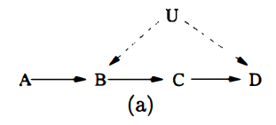
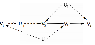
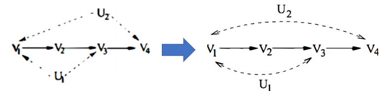
예를 들어, 아래의 두 causal model은 같은 conditional independence among the observed variables를 갖는다.

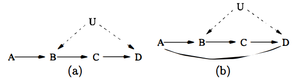
그러나 Verma의 functional constraint에 의해서 이 둘 사이에서 구분할 수 있다.

Conditional indenpendence relationship에만 의존한 structure-learning은 두 모델을 구분할 수 없다.

---

Causal model with hidden variable에 의해 암시된 functional constraint를 찾는
대수적(not graphical) 메소드는 Geiger, 1998~9에서 나왔었다.

그러나 이들은 계산량이 많아서 small network with small parameters에 국한됐다.

---

이 논문은 F constraint를 graph를 기반으로 체계적으로 찾아내는 procedure를 보이겠다.

2. Bayesian Networks with Hidden Variables

Bayesian network는 joint probability distribution의 factorization을 주장한다.

$$P(v)=\prod_{i} P\left(v_{i} \mid p a_{i}\right)$$

만약 몇몇 변수들이 unobserved일 때, 변수를 $V=\left\{V_{1}, \ldots, V_{n}\right\} \text { and } U=\left\{U_{1}, \ldots, U_{n^{\prime}}\right\}$로 나누면,

observed probability distribution은 다음과 같다.

$$\begin{aligned} P(v) &=\sum_{u} \prod_{\left\{i \mid V_{i} \in V\right\}} P\left(v_{i} \mid p a_{v_{i}}\right) \prod_{\left\{i \mid U_{i} \in U\right\}} P\left(u_{i} \mid p a_{u_{i}}\right) \\ &= \sum_{u^{\prime}} \prod_{V_{i} \in V} P\left(v_{i} \mid p a_{v_{i}}\right) \prod_{U_{i} \in U^{\prime}} P\left(u_{i} \mid p a_{u_{i}}\right) \quad \text{where $U' = An(V) \cap U$} \end{aligned}$$

$V$의 ancestor가 아닌 unobserved는 joint distribution에서 다 쳐낼 수 있으므로, 앞으로 이들은 없다고 가정하겠다.

---

For any $S \subseteq V$

$$Q[S](v) :=\sum_{u} \prod_{\left\{i \mid V_{i} \in S\right\}} P\left(v_{i} \mid p a_{v_{i}}\right) \prod_{\left\{i \mid U_{i} \in U\right\}} P\left(u_{i} \mid p a_{u_{i}}\right)$$

$Q[S](v)$의 해석: $S$이외의 변수에 $v \setminus s$의 intervention을 줬을 때 $S$가 $s$의 값을 가질 확률

Note that

1. $Q[V](v)=P(v)$
2. $Q[\emptyset](v)=1$

위의 joint distribution을 $U$를 포함한 텀과 아닌 텀을 나눠보면, $P(a, b, c, d)=P(a) P(c \mid b) Q[\{B, D\}]$ 임을 알 수 있고

$$\begin{aligned} Q[\{B, D\}] &= \sum_{u} P(b \mid a, u) P(d \mid c, u) P(u) \quad \text{by def} \\ &= \frac{P(a, b, c, d)}{P(a) P(c \mid b)} \quad \because \text{derived factorization} \\ &= \frac{P(a, b, c, d)}{P(a \mid b) P(c \mid a, b)} \times \frac{p(b\mid a)}{p(b)} \quad \text{by Bayes' rule} \\ &= \frac{P(a, b, c, d)}{P(a, c \mid b)} \times \frac{p(b\mid a)}{p(b)} \\ &= \frac{P(a, c, d\mid b) p(b) }{P(a, c \mid b)} \times \frac{p(b\mid a)}{p(b)} \\ &= P(d \mid a, b, c) \times P(b \mid a) \\ \\ Q[\{D\}]&= \sum_{u} P(d \mid c, u) P(u) \quad \text{by def} \\ &=\sum_{b} Q[\{B, D\}] \quad \text{fortunate observation!} \\ & =\sum_{b} P(d \mid a, b, c) P(b \mid a) \end{aligned}$$

애초에 $Q[\{D\}]$는 $c$의 함수이기에 $\sum_{b} P(d \mid a, b, c) P(b \mid a)$이 $a$에 의존하지 않는다는 것을 알게된다.

이러한 functional constraint를 찾는 것은 c-factor $Q[\{B, D\}]$와 $Q[\{D\}]$를 $P(v)$로 표현하는 능력에 달려있다.

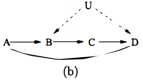
하지만 이 경우엔 애초에 $Q[\{D\}] = \sum_{u} P(d \mid c, a, u) P(u)$ $a, c, d$의 함수라서 functional constraint는 없다.

---

$Q[S](v)$는 $V$의 subset의 함수이고 $P(v)$로 계산이 가능하다면, 이로부터 CI 혹은 F constraint가 유도될 수 있다.

이 논문에선 $P(v)$로 계산이 가능한 $Q[S]$를 찾는 법을 보이게 된다.

---

For any $C$, let

• $G_{C} :=$ the subgraph of $G$ composed only of $C$
• $An^u(C) := An(C) \cap U$ ; $C$의 조상 중에서 hidden variable
• $G(C) := G_{C \cup U(C)}$

For any $S \subseteq V$, let

• $U(S) := An^u(S)_{G_{S\cup U}}$ ; $S$와 $U$로 구성된 subgraph에서 $S$의 조상 중에서 hidden variable

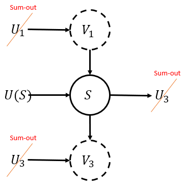
$Q[S]$에서 $G_{S \cup U}$에서 $S$의 조상이 아닌 $U_i$는 $p(v_i \mid pa_{v_i})$ 등장하지 않아 sum-out되기 마련이다.

이 논문에서 sum-out은 진짜 많이 사용하는 테크닉이다.

고려하고 있는 graph에서 해당 노드가 말단노드인 경우, sum을 하면 product에서 없어진다.

• $Q[S]=\sum_{u(S)\left\{i \mid V_{i} \in S\right\}} P\left(v_{i} \mid p a_{v_{i}}\right) \prod_{\left\{i \mid U_{i} \in U(S)\right\}} P\left(u_{i} \mid p a_{u_{i}}\right)$
  • $Q[S]$는 $S$와 $Pa^v(S)$와 $Pa^v\left(U(S) \right)$의 함수이다.
  • 이를 좀 더 명료하게 표현하기 위해
  • If ${}^\exists \text{directed path }V_i \rightarrow V_j$ s.t. all the internal nodes are hidden variables, $V_i$ is an effective parent of $V_j$
  • Let $Pa^+(S)$ denote $S \cup \{ V_i \in V \mid \text{$V_i$ is an effective parent of $S$}\}$
  • Then, $Q[S]$ is a function of $Pa^+(S)$.

만약 $Q[S](t)$이 $P(v)$로 표현될 수 있다면, $Q[S](t)$는 $T’ \supset T$의 함수이다.

결국, $Q[S]$의 $P(v)$ 표현에서 $t’ \setminus t$에 의해 값이 변하지 않는다는 constraint가 생긴다.

Constraint는 F constraint이거나 CI constraint가 될 것이다.

---

For any $C$, let

• $A n^{v}(C)=A n(C) \cap V$ ; $C$의 조상 중에서 observed variable
• $D e^{v}(C) = [ De(C) \cap V] \cup V(C)$ ; $C$ 혹은 $C$의 후손 중에서 observed variable

Let

• $A \subseteq V$ is an ancestral set if $A= An^v(A)$
• $A \subseteq V$ is a descendent set if $A= De^v(A)$

---

Lemma 1 (sum-out의 set버전이다.)

​ Let $W \subseteq C \subseteq V$

​ Let $W’ = C \setminus W$

​ If $W$ is an ancestral set in $G(C)$, then $\sum_{w^{\prime}} Q[C]=Q[W]$

​ Equivalently, if $W’$ is a descendent set in $G(C)$, then $\sum_{w^{\prime}} Q[C]=Q[W]$

(Proof)

​ 증명을 하기 전에 테크닉적인 부분을 짚고 넘어가자.

​ 일단 sum-out이 되기 위해선 $\prod $

$$\begin{aligned} \sum_{w^{\prime}} Q[C] &=\sum_{w^{\prime}} \sum_{u(C)} \prod_{V_{i} \in C} P\left(v_{i} \mid p a_{v_{i}}\right) \prod_{U_{i} \in U(C)} P\left(u_{i} \mid p a_{u_{i}}\right) \\ &= \sum_{A n^{u}(W)_{G(C)}} \prod_{V_{i} \in W} P\left(v_{i} \mid p a_{v_{i}}\right) \prod_{U_{i} \in A n^{u}(W)_{G(C)}} P\left(u_{i} \mid p a_{u_{i}}\right) \\ &= \sum_{U(W)} \prod_{V_{i} \in W} P\left(v_{i} \mid p a_{v_{i}}\right) \prod_{U_{i} \in A n^{u}(W)_{G(C)}} P\left(u_{i} \mid p a_{u_{i}}\right) \\ &= Q[W] \end{aligned}$$

• 첫번째 등식은 그냥 정의이다.
• 두번째 등식은 $W’$이 ancestral set의 여집합 느낌이라 topological order에 맞춰서 sum-out하다 보면 이 꼴이 될 것임은 명백하다.
• 세번째 등식은 $W$이 ancestral set이기 떄문에 $A n^{u}(W)_{G(C)}=A n^{u}(W)_{G_{W \cup U}}=U(W)$ 이다.
• 네번째 등식은 그냥 정의이다.

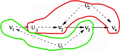
3. C-components

$$\begin{aligned} P(v_1, v_2, v_3, v_4) = &\sum_{u_1, u_2, u_3} \prod_{\left\{i \mid V_{i} \in V\right\}} P\left(v_{i} \mid p a_{v_{i}}\right) \prod_{\left\{i \mid U_{i} \in U\right\}} P\left(u_{i} \mid p a_{u_{i}}\right) \\ = &\left(\sum_{u_{1}} P\left(v_{1} \mid u_{1}\right) P\left(v_{3} \mid v_{2}, u_{1}\right) P\left(u_{1}\right)\right) \\ & \left(\sum_{u_{2}, u_{3}} P\left(v_{2} \mid u_{2}, u_{3}\right) P\left(v_{4} \mid v_{3}, u_{2}\right) P\left(u_{2}\right) P\left(u_{3} \mid v_{1}\right)\right) \\ & =Q\left[\left\{V_{1}, V_{3}\right\}\right] Q\left[\left\{V_{2}, V_{4}\right\}\right] \end{aligned}$$

위의 decomposition의 중요성은 각 $Q$들이 $P(v)$로 계산이 가능하다는 것이다.

이번 섹션에선 Tian & Pearl 2002의 non-root $U$를 허용하는 더 일반적인 graphical criterion을 보이겠다.

---

Joint distribution에 대한 아래의 decomposition을 확인해보자겠다.

$$P(v)=\prod_{j}\left(\sum_{n,} \prod_{V_{i} \in S_{j}} P\left(v_{i} \mid p a_{v_{i}}\right) \prod_{U_{i} \in N_{j}} P\left(u_{i} \mid p a_{u_{i}}\right)\right) \prod_{V_{i} \in S^{0}} P\left(v_{i} \mid p a_{v_{i}}\right)$$

where

• $S^0$ is the set of observed variables having no hidden parents
• $N_k$ is the set of hidden variables s.t.
  • $^\forall U_i \& U_j \in N_k$, they have a common child
  • or
  • $^ \exists $edge between $(U_i, U_j)$
• $S_j$ is the set of observed variables whose hidden parents are in $N_j$

Note that

1. $U_i$와 $U_j$ 사이엔 적어도 하나의 path가 있다. s.t.

   • $U$로만 이뤄졌거나
   • path상의 observed node가 모두 $\rightarrow V_{l} \leftarrow$ 꼴이거나

2. $ \{ \{S_i^0 \}_i, \{ S_i\}_i \}$은 $V$의 partition이다.

   Partition의 각 set을 c-component라고 부르겠다.

3. $U_k \not \in N_j$ 는 inner term $\prod_{V_{i} \in S_{j}} P\left(v_{i} \mid p a_{v_{i}}\right) \prod_{U_{i} \in N_{j}} P\left(u_{i} \mid p a_{u_{i}}\right)$ 에 등장하지 않는다.

4. c-component의 root node는 무조건 hidden이다.

2와 3을 종합해보면 decomposition이 확인할 수 있다.

Tian & Pearl 2002에서 특수 케이스에 대해 다뤘었다.

---

추가로,

$$\begin{aligned} Q\left[S_{j}\right] &=\sum_{u} \prod_{\left\{i \mid V_{i} \in S_{j}\right\}} P\left(v_{i} \mid p a_{v_{i}}\right) \prod_{\left\{i \mid U_{i} \in U\right\}} P\left(u_{i} \mid p a_{u_{i}}\right) \\ &=\sum_{n_{j}} \prod_{V_{i} \in S_{j}} P\left(v_{i} \mid p a_{v_{i}}\right) \prod_{U_{i} \in N_{j}} P\left(u_{i} \mid p a_{u_{i}}\right) \sum_{u \setminus n_{j}} \prod_{U_{i} \in U \setminus N_{j}} P\left(u_{i} \mid p a_{u_{i}}\right) \\&= \sum_{n_{j}} \prod_{V_{i} \in S_{j}} P\left(v_{i} \mid p a_{v_{i}}\right) \prod_{U_{i} \in N_{j}} P\left(u_{i} \mid p a_{u_{i}}\right) \end{aligned}$$

이므로 $P(v)=Q[V]=\prod_{i} Q\left[S_{i}\right]$ c-component들의 c-factor로 분해됨을 알 수 있다.

where $S_{1}, \ldots, S_{k}$ is the c-components of $V$

---

C-factor로의 분해가 중요한 이유는 이들이 $P(v)$로 계산이 가능하기 때문이다.

Lemma 2와 Corollary 1을 보자.

---

Lemma 2 (Tian & Pearl 2002에서 $H = V$로 두고 hidden node는 root node임을 가정하였을 때 증명했었다. 결국 렘마의 의미는 subgraph의 c-factor마저 identifiable하다이다.)

​ Let $H \subseteq V$

​ Let $H_{1}, \ldots, H_{l}$ be the c-components in the subgraph $G(H) = G_{H \cup U(H)}$

​ [1] : Then, $Q[H]=\prod_{i} Q\left[H_{i}\right]$

​ Let $k$ be the number of variables in $H$

​ Let a topological order of the variables in $H$ be $V_{h_{1}}<\cdots< V_{h_k}$ in $G(H)$

​ Let $H^{(i)}=\left\{V_{h_{1}}, \ldots, V_{h_{i}}\right\}$ and $H^{(0)} = \emptyset$

​ [2] : Then, $Q\left[H_{j}\right] =\prod_{\left\{i \mid V_{h_{i}} \in H_{j}\right\}} \frac{Q\left[H^{(i)}\right]}{Q\left[H^{(i-1)}\right]}$ where $Q\left[H^{(i)}\right] =\sum_{h \backslash h^{(i)}} Q[H] $

$Q\left[H^{(i)}\right] =\sum_{h \backslash h^{(i)}} Q[H] $이 Lemma 1의 inverse임을 인지하여야 함!

​ [3] : Then, $\frac{Q\left[H^{(i)}\right]}{Q\left[H^{(i-1)}\right]}$ is a function only of $P a^{+}\left(T_{i}\right)$ where $T_i$ is a c-component of $G(H^{(i)})$ that contains $V_{h_i}$

$T_i$를 점점 커지는 $G(H)$에서 최근에 추가된 노드가 속한 c-component를 생각하면 직감적

(Proof)

[1]

​ $\begin{aligned} Q[H] &=\sum_{u(H)\left\{i \mid V_{i} \in H\right\}} P\left(v_{i} \mid p a_{v_{i}}\right) \prod_{\left\{i \mid U_{i} \in U(H)\right\}} P\left(u_{i} \mid p a_{u_{i}}\right) \\ &= P(v)_{G(H)}\end{aligned}$

​ 즉, $G(H)$의 joint distribution이고 이는 $G(H)$에서의 c-component들로 분해가 가능하다.

[2, 3]

증명을 시작하기에 앞서 $H^{(i)}$는 ancestral set임을 인지하여 Lemma 1이 적용될 수 있다는 걸 인지하라.

Base

​ Let $H \subseteq V$ with $H = H_1 = \{ V_{h_1}\}$

​ It is clear that $Q[H_1] = Q[H^{(1)}] =\sum_{h \backslash h^{(i)}} Q[H_1] $.

​ Since $Q[H_1]$ is a function of $Pa^{+}(H_1)$,

$$\text{$Q\left[H^{(1)}\right]=\sum_{h \backslash h^{(i)}} Q[H_1] \quad $ is also a function only of $Pa^{+}(H_1)$}$$

Hypothesis :

​ Let $H \subseteq V$ with $H = \{ V_{h_1}, \cdots, V_{h_k}\}$

​ Assume that

1. all $Q\left[H_{j}\right] =\prod_{\left\{i \mid V_{h_{i}} \in H_{j}\right\}} \frac{Q\left[H^{(i)}\right]}{Q\left[H^{(i-1)}\right]}$
2. $\frac{Q\left[H^{(i)}\right]}{Q\left[H^{(i-1)}\right]}$ is a function only of $P a^{+}\left(T_{i}\right)$ for $i=1, \cdots ,k$.

Induction

​ Let $H \subseteq V$ with $H = \{ V_{h_1}, \cdots, V_{h_k}, V_{h_{k+1}}\}$.

​ Let $H_{1}, \cdots, H_{m}, H^{\prime}$ is the c-components of $G(H)$ where $V_{h_{k+1}} \in H^{\prime}$.

​ Then, we have $\begin{aligned}Q[H] &=Q\left[H^{(k+1)}\right] \\&=Q\left[H^{\prime}\right] \prod_{i} Q\left[H_{i}\right] \quad \text{by Lemma 2 [1]}\end{aligned}$

​ Then,

$$\begin{aligned} \sum_{v_{h_{k+1}}}Q[H] &=Q\left[H^{(k)}\right] \quad \text{by Lemma 1} \\&= \left(\sum_{v_{h_{k+1}}}Q\left[H^{\prime}\right] \right) \prod_{i} Q\left[H_{i}\right]\end{aligned}$$

​ It is clear that each $H_i $, $i=1, \cdots, m$, is a c-component of the subgraph $G[H^{(k)}]$.

​ Therefore, by hypothesis, we have

$$Q\left[H_{j}\right] =\prod_{\left\{i \mid V_{h_{i}} \in H_{j}\right\}} \frac{Q\left[H^{(i)}\right]}{Q\left[H^{(i-1)}\right]} \quad \text{for $j=0, 1, \cdots, m$}$$

​ where $Q\left[H^{(i)}\right]=\sum_{h^{(k)} \backslash h^{(i)}} Q\left[H^{(k)}\right]=\sum_{h \backslash h^{(i)}} Q[H]$

​ Hence,

$$\begin{aligned} Q\left[H^{\prime}\right] & = \frac{Q[H^{(k+1)}]}{\prod_{i=1} ^m Q[H_i]} \\ &= \frac{\prod_{i=1}^{k+1}\left[ \frac{Q\left[H^{(i)}\right]}{Q\left[H^{(i-1)}\right]} \right]}{\prod_{i=1} ^m Q[H_i]} \\ & = \frac{\prod_{i=1}^{k+1}\left[ \frac{Q\left[H^{(i)}\right]}{Q\left[H^{(i-1)}\right]} \right]}{\prod_{i: V_{h_i} \in H_1 \cup \cdots \cup H_m} \left [\frac{Q\left[H^{(i)}\right]}{Q\left[H^{(i-1)}\right]}\right ]} \\ &= \prod_{\left\{i \mid V_{h_{i}} \in H^{\prime}\right\}} \frac{Q\left[H^{(i)}\right]}{Q\left[H^{(i-1)}\right]} \end{aligned}$$

​ Now, we want to show that $\frac{Q[H^{(k+1)}]}{Q[H^{(k)}]}$ is a function of $Pa^+(H’)$

​ Fact : $Q[H’]$ is a function of $Pa^+(H’)$.

​ Hypothesis : For $i \in \{i : V_{h_i} \in H’ \setminus \{ V^{k+1}\} \}$, $ \frac{Q\left[H^{(i)}\right]}{Q\left[H^{(i-1)}\right]}$ is a function of $Pa^+(T_i) \subset Pa^+(H’)$

​ Hence, $\frac{Q[H^{(k+1)}]}{Q[H^{(k)}]} = Q[H’] \quad / \quad \prod_{i \in \{i : V_{h_i} \in H’ \setminus \{ V^{k+1}\} \}} \frac{Q\left[H^{(i)}\right]}{Q\left[H^{(i-1)}\right]}$ is also a function of $Pa^+(H’)$

---

Corollary 1

​ Let $V$ be partitioned into c-components $S_1, \cdots, S_k$

​ Let a topological order of $V$ be $V_{1}<\ldots<V_{n}$

​ Let $V^{(i)} = \{V_1, \cdots, V_i \}$ and $V^{(0)}= \emptyset$

​ Then,

• $P(v) = \prod_i Q[S_i]$
• $Q[S_j] = \prod_{i : V_i \in S_j} P(v_i \mid v^{(i-1)})$
• $P(v_i \mid v^{(i-1)}) = P(v_i \mid Pa^+ (T_i) \setminus \{ V_i\})$

(Proof)

​ 첫번째껀 $H = V$로 두고 Lemma 2 [1] 적용

​ 두번째껀 $\frac{Q\left[H^{(i)}\right]}{Q\left[H^{(i-1)}\right]} = P(v_i \mid v^{(i-1)})$이므로 $Q[S_j] = \prod_{i : V_i \in S_j} P(v_i \mid v^{(i-1)})$

​ 세번째껀 $P(v_i \mid v^{(i-1)}) = \frac{Q\left[H^{(i)}\right]}{Q\left[H^{(i-1)}\right]} $ 이고 Lemma 2 [3]에서 $\frac{Q\left[H^{(i)}\right]}{Q\left[H^{(i-1)}\right]}$이 function ofx $P a^{+}\left(T_{i}\right)$ 임을 보였다.

4. Finding Constraints

Lemma 1, 2와 Corollary 1을 갖고서, network structure에 의해 부과된 constraint를 체계적으로 찾을 수 있다.

4.1 Examples

$V$ is decomposed to two c-components $\{ V_1, V_3\}, \{V_2, V_4 \}$

The topological order of $V$ in $G$ is $V_{1}<V_2 < V_3 < V_{4}$

Applying corollary 1, we can get

$$\begin{aligned} Q\left[\left\{V_{1}, V_{3}\right\}\right]\left(v_{1}, v_{2}, v_{3}\right) &=P\left(v_{3} \mid v_{2}, v_{1}\right) P\left(v_{1}\right) \\ Q\left[\left\{V_{2}, V_{4}\right\}\right]\left(v_{1}, v_{2}, v_{3}, v_{4}\right) &=P\left(v_{4} \mid v_{3}, v_{2}, v_{1}\right) P\left(v_{2} \mid v_{1}\right) \end{aligned}$$

이들 자체적으론 $P(v)$에 constraint를 주진 않는다. 추가적으로,

$$\begin{aligned} Q[V_4] &= Q[V_4](v_3, v_4) \quad \because Pa^+(V_4) = \{ V_3, V_4\} \\ &= \sum_{v_2} Q\left[\left\{V_{2}, V_{4}\right\}\right]\left(v_{1}, v_{2}, v_{3}, v_{4}\right) \quad \because \text{Lemma 1} \\ &=\sum _{v_2} P\left(v_{4} \mid v_{3}, v_{2}, v_{1}\right) P\left(v_{2} \mid v_{1}\right) \\ &= f(v_1, v_2, v_4) \end{aligned}$$

$Q[V_4]$에 의해서, $f(v_1, v_2, v_4)$가 $v_1$에 의존하지 않는다고 $P(v)$에 constraint가 들어간다.

참고로 나머지 $Q[V_1], Q[v_2], Q[V_3]$는 constraint를 부과하지 않는다.

---

$G$

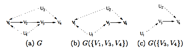
• has two c-components $\{ V_2\}, \{V_1, V_3, V_4 \} =: S$
• has a topological order $V_1 < V_2 < V_3 < V_4$
• Applying corollary 1,
  • $Q[V_2] (v_1, v_2) = P(v_2 \mid v_1)$
  • $Q[S](v) = P\left(v_{4} \mid v_{3}, v_{2}, v_{1}\right) P\left(v_{3} \mid v_{2}, v_{1}\right) P\left(v_{1}\right)$

$G(S) = G\left(\left\{V_{1}, V_{3}, V_{4}\right\}\right)$

• $H:= S \setminus \{ V_1\} = \{ V_3, V_4\}$

• $$\begin{aligned} Q[H]\left(v_{2}, v_{3}, v_{4}\right) &= \sum_{v_1} Q[S] \quad \because \text{Lemma 1} \\ &= \sum_{v_{1}} P\left(v_{4} \mid v_{3}, v_{2}, v_{1}\right) P\left(v_{3} \mid v_{2}, v_{1}\right) P\left(v_{1}\right) \end{aligned}$$

$G(H) = G\left(\left\{V_{3}, V_{4}\right\}\right)$

• has two c-components $\left\{V_{3}\right\}, \left\{V_{4}\right\}$

• has a topological order $V_3 < V_4$

• $$\begin{aligned} Q[H]\left(v_{2}, v_{3}, v_{4}\right) &= Q[\{V_3\}] Q[ \{V_4\}] \quad \because \text{Lemma 2} \\ \\ Q[\{V_3\}](v_2, v_3) &= \sum_{v_4} Q[H] = \sum_{v_{1}} P\left(v_{3} \mid v_{2}, v_{1}\right) P\left(v_{1}\right) \quad \because \text{Lemma 1} \\ \\ Q\left[\left\{V_{4}\right\}\right]\left(v_{3}, v_{4}\right)&=\frac{Q[H]}{\sum_{v_{4}} Q[H]} \quad \because \text{by the first equation} \\ &=\frac{\sum_{v_{1}} P\left(v_{4} \mid v_{3}, v_{2}, v_{1}\right) P\left(v_{3} \mid v_{2}, v_{1}\right) P\left(v_{1}\right)}{\sum_{v_{1}} P\left(v_{3} \mid v_{2}, v_{1}\right) P\left(v_{1}\right)} \end{aligned}$$

• 결국, $P(v)$에 RHS가 $v_2$에 의존하지 않는다는 constraint를 준다.

---

두 예제로 부터, Lemma 1과 Lemma 2를 번갈아 적용하면 constraint를 찾을 수도 있다는 걸 발견했다.

이를 체계적으로 하는 과정을 소개하겠다.

4.2 Identifying constraints systematically

Let a topological order over $V$ be $V_{1}<\ldots<V_{n}$.

Let $V^{(i)} = \left\{V_{1}, \ldots, V_{i}\right\}$ for $i=1, \cdots, n$

for i = 1:n
	do A1
	do A2

A1

• Assume $G(V^{(i)})$ has more than one c-components ; (두 개 이상의)
• Let $V_i \in S_i \in \{\text{c-components of }G(V^{(i)}) \}$
• Then, by corollary 1,
  • $Q[S_i]$ is computable from $P(v)$
  • $P(v_i \mid v^{(i-1)}) = P(v_i \mid Pa^+ (S_i) \setminus \{ V_i\})$ implies conditional independence constraint
    • $V_i \perp \Big[ V^{(i)} \setminus Pa^+(S_i) \Big ] \mid \Big[ Pa^+(S_i)\setminus\{ V_i \} \Big]$

A2

• Consider $Q[S_i]$ in the subgraph $G(S_i)$

• For each descendent set $D \in S_i$ in $G(S_i)$ that does not contain $V_i$,

  $$\sum_{d} Q\left[S_{i}\right]=Q\left[S_{i} \backslash D\right] \quad \because \text{by Lemma 1}$$

  • 왼쪽 식은 $Pa^+(S_i) \setminus D$의 함수이고 오른쪽 식은 $P a^{+}\left(S_{i} \setminus D\right)$의 함수이다.

  • $ \Big[P a^{+}\left(S_{i} \setminus D\right) \Big] \subseteq Pa^+(S_i) \setminus D$ 임은 명백하다.

    effective parent of $D$가 effective parent of $(S \setminus D)$에 속하지 않을 때 차이가 있다.

  • 결국 $\Big [Pa^+(S_i) \setminus D \Big] \setminus \Big[P a^{+}\left(S_{i} \setminus D\right) \Big] \neq \emptyset$일 때, $P(v)$에 CI constraint를 준다.

    • $\sum_{d} Q\left[S_{i}\right]$ is independent of $\Big [Pa^+(S_i) \setminus D \Big] \setminus \Big[P a^{+}\left(S_{i} \setminus D\right) \Big]$

• Let $D’ = S_i \setminus D$

• If $G(D’)$ has more than one c-components, (else just $D’=E_i$, skip )

  • let $V_i \in E_i$ where $E_i$ is the c-component of $G(D’)$
  • By Lemma 2, $\left \{\begin{array}{l}
    Q[E_i] \text{ is computable from } Q[D’] \\
    Q[D’] = Q[E_i] \prod_{ C \in \{\text{other c-comp}\}} Q[C]
    \end{array}\right.$
  • By Lemma 1, $\begin{aligned}Q[D’ \setminus \{ V_i\}] &= \sum_{v_i} Q[D’] \\&= \sum_{v_i}Q[E_i] \prod_{ C \in \{\text{other c-comp}\}} Q[C] \\ &=Q[E_i \setminus \{ V_i\}] \prod_{ C \in \{\text{other c-comp}\}} Q[C] \end{aligned}$
  • Therefore, $\frac{Q[D’]}{Q[D’ \setminus \{V_i\}]} = \frac{Q\left[D^{\prime}\right]}{\sum_{v_{i}} Q\left[D^{\prime}\right]} = \frac{Q[E_i]}{Q[E_i \setminus \{ V_i\}]}$ is a function only of $Pa^+(E_i)$
  • 결국 $P a^{+}\left(D^{\prime}\right) \backslash P a^{+}\left(E_{i}\right) \neq \emptyset$ 일 때, $P(v)$에 F constraint를 준다.

---

위의 알고리즘은 체계적으로 constraint를 찾는 과정을 준다.

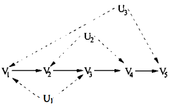
$i=1,\cdots, 4$까진 아래의 조건이 만족된다.

1. $V^{(i)} = Pa^+(S_i)$
2. $Pa^+(S_i) \setminus D = Pa^+(S_i \setminus D)$
3. $Pa^+(D’) = Pa^+(E_i)$

$i=5$일 때

• $S_i = \{ V_1, V_3, V_5\}$이다.
• $G(S_i)$의 descendent set $D = \{ V_1\} , \{ V_3\}, \{ V_1,V_3\}$이 있다.

$D$	$\{V_1\}$	$\{V_3\}$	$\{ V_1, V_3\}$
$Pa^+(S_i \setminus D)$	$\{ V_2, V_3, V_4, V_5\}$	$\{ V_1, V_4, V_5\}$	$\{ V_4, V_5\}$
$Pa^+(S_i)\setminus D)$	$\{V_2, V_3, V_4, V_5\}$	$\{V_1, V_2, V_4, V_5\}$	$\{ V_2, V_4, V_5\}$
$D’$	$\{ V_3, V_5\}$	$\{ V_1, V_5\}$	$\{ V_5\}$
$E_i$	$\{ V_5\}$	$\{V_1, V_5\}$	$\{ V_5\}$
$Pa^+(D’)$	$\{ V_2, V_3, V_4, V_5\}$	$\{V_1, V_4, V_5 \}$	$\{ V_4, V_5\}$
$Pa^+(E_i)$	$\{ V_4, V_5\}$	$\{V_1, V_4, V_5\}$	$\{ V_4, V_5\}$

$D = V_1$일 때

$$Q\left[\left\{V_{3}, V_{5}\right\}\right]\left(v_{2}, v_{3}, v_{4}, v_{5}\right)=\sum_{v_{1}} P\left(v_{5} \mid v_{4}, v_{3}, v_{2}, v_{1}\right) P\left(v_{3} \mid v_{2}, v_{1}\right) P\left(v_{1}\right)$$

는 아무런 constraint를 주지 않는다.

$$Q\left[\left\{V_{5}\right\}\right]\left(v_{4}, v_{5}\right)=\frac{Q\left[\left\{V_{3}, V_{5}\right\}\right]}{\sum_{v_{5}} Q\left[\left\{V_{3}, V_{5}\right\}\right]} = \frac{\sum_{v_{1}} P\left(v_{5} \mid v_{4}, v_{3}, v_{2}, v_{1}\right) P\left(v_{3} \mid v_{2}, v_{1}\right) P\left(v_{1}\right)}{\sum_{v_{1}} P\left(v_{3} \mid v_{2}, v_{1}\right) P\left(v_{1}\right)}$$

는 RHS가 $v_2, v_3$에 독립이라고 constraint를 준다.

$D = V_3$일 때

$$Q\left[\left\{V_{1}, V_{5}\right\}\right]\left(v_{1}, v_{4}, v_{5}\right)=\sum_{v_{3}} P\left(v_{5} \mid v_{4}, v_{3}, v_{2}, v_{1}\right) P\left(v_{3} \mid v_{2}, v_{1}\right) P\left(v_{1}\right)$$

는 RHS가 $v_2,$에 독립이라고 constraint를 준다.

$D = \{V_1, V_3\}$일 때

$$Q\left[\left\{V_{5}\right\}\right]\left(v_{4}, v_{5}\right) =\sum_{v_{1}, v_{3}} P\left(v_{5} \mid v_{4}, v_{3}, v_{2}, v_{1}\right) P\left(v_{3} \mid v_{2}, v_{1}\right) P\left(v_{1}\right)$$

는 RHS가 $v_2$에 독립이라고 constraint를 준다.

이는 $D=V_1$일 때 얻은 constraint와 똑같다. (summation $v_3$ 해보면 앎)

5. Projection to Semi-Markovian Models

Semi-Markovian Model은 hidden variable이 root node이며 두개의 자식만 갖는 Bayesian network를 말한다.

SMM이 일반적인 Bayesian network with hidden variables보다 작업하기 쉽다.

BN with hidden variables가 SMM with same set of constraints on $P(v)$으로 변환될 수 있음을 보이겠다.

5.1 Semi-Markovian models

	BN	SMM
$P(v)$	$\sum_{u} \prod_{\left\{i \mid V_{i} \in V\right\}} P\left(v_{i} \mid p a_{v_{i}}\right) \prod_{\left\{i \mid U_{i} \in U\right\}} P\left(u_{i} \mid p a_{u_{i}}\right)$	$\sum_{u} \prod_{\left\{i \mid V_{i} \in V\right\}} P\left(v_{i} \mid p a_{v_{i}}\right) \prod_{\left\{i \mid U_{i} \in U\right\}} P\left(u_{i}\right)$
$Q[S]$	$\sum_{u} \prod_{\left\{i \mid V_{i} \in S\right\}} P\left(v_{i} \mid p a_{v_{i}}\right) \prod_{\left\{i \mid U_{i} \in U\right\}} P\left(u_{i} \mid p a_{u_{i}}\right)$	$\sum_{u} \prod_{\left\{i \mid V_{i} \in S\right\}} P\left(v_{i} \mid p a_{v_{i}}\right) \prod_{\left\{i \mid U_{i} \in U\right\}} P\left(u_{i} \right)$

편의를 위해 더 이상 hidden variable을 node로 표기하지 않는다.

그 경우 Bidirected path는 Bidirected edge만으로 이어진 path를 의미한다.

C-component는 Bidirected path상의 노드들로 간단하게 정의된다.

$Pa(S) := S \cup \Big [ \cup_{S_i \in S }\{ Pa(S_i) \} \Big ]$

---

이러한 SMM의 셋팅에서 Lemma 1, Lemma 2의 statement에서

• $G(C) \Rightarrow G_C$, $G(H) \Rightarrow G_H$
  • 더 이상 unobserved node를 node취급을 안하고 confounding arc로 처리함
• $Pa^+ (\cdot) \Rightarrow Pa(\cdot)$
  • unobserved node는 root node이므로 effective parent와 parent는 동일한 말이다.
  • $Pa$도 이제 자기 자신을 포함함

5.2 Projection

Bayesian network with hidden variables를 Semi-Markovian Model로 project해보겠다.

Definition 1

​ Let $PJ(G, V)$ be the projection of DAG $G$ over $V\cup U\Rightarrow V$ that follows

1. Add each variable in $V$
2. ${}^\forall \text{pair }X,Y \in V$, if there is a edge btw $X$ and $Y$, then add the edge
3. ${}^\forall \text{pair }X,Y \in V$, if there is a directed path $X\rightarrow Y$ in $G$ s.t. every internal node is in $U$, then add the edge
4. ${}^\forall \text{pair }X,Y \in V$, if there is a divergent path btw $X$ and $Y$ s.t. every internal node is in $U$ then add bidirected edge btw $X$ and $Y$

divergent path는 $\left(X \leftarrow - U_{i}- \rightarrow Y\right)$ 이런 모양이다.

4.2에서 소개한 알고리즘이 $G$와 $PJ(G,V)$에서 찾는 set of constraints on $P(v)$이 서로 같다는 것을 보이기 위해선

$${}^{\forall}H \subseteq V, \text{$G$ and $PJ(G,V)$ have }\left\{\begin{array}{l} \text{the same arguments for $Q[H]$} \\ \text{the same topological relations over $H$}\\ \text{the same sets of c-components} \end{array}\right.$$

Lemma 3

​ ${}^\forall H \subseteq V$, $Pa^+(H)$ in $G$ is equal to $Pa(H)$ in $PJ(G, V)$

(Proof)

​ 이는 명백하다.

Lemma 4

​ Let $H \subseteq V$

​ Let $V_i, V_j \in H$

• $V_i \in An(V_j)$ in $G(H)$

  if and only if

• $V_i \in An(V_j)$ in $P(G, V)_H$

(Proof)

​ 이는 Verma, 1993에서 증명됐다.

Lemma 5

​ ${}^\forall H \subseteq V$, $G(H)$ is partitioned into the same set of c-components as $PJ(G, V)_H$

(Proof)

​ 이는 appendix에 있는데 생략하겠다.

---

결국, SMM으로 projection을 하고나서 $P(v)$에 걸리는 constraint를 찾아도 된다.

6. Conclusion

Constraint를 찾아서 structure의 유효성을 검증하는 데 사용할 수 있다.

아쉽게도, 우리의 알고리즘이 모든 functional constraint를 찾는다는 보장은 없다.