Reliable Decision Support using Counterfactual Models

0. Abstract

Decision maker는 어떤 action을 취했을 때 일어날 법한 것을 estimate해야한다.

예를 들어, 환자를 치료하지 않기로 결정하면 그들은 어느 정도의 확률로 죽을까? 를 고민하게 된다.

이 경우에 practitioner들은 supervised learning algorithm으로 outcome을 예측하는 predictive model을 보통 학습한다.

하지만, 이러한 방식은 unreliable하고 가끔은 위험할 수도 있다.

왜냐면 supervised learning algorithm은 training data에 존재했던 policy에 민감하기 때문이다.

결국, 이는 model이 일반화될 수 없는 관계를 잡게 되버린다.

이 문제를 해결하기 위해

• 기존의 policy 하에서 outcome을 예측하는 대신에
• counterfactual outcome을 예측하는 learning objective를 제안할 것이다.

Temporal setting에서 decision making을 지원하기 위해서 Counterfactual Gaussian Process를 도입하게 될 것이다.

이는 action들의 sequence를 받고서, continuous-time 상에서 counterfactual future regression을 예측한다.

1. risk prediction을 제공하고
2. 각 개인 별 treatment planning을 위한 “what if”에 대한 답을 줄 수 있다.

1. Introduction

Decision maker는 어떤 action을 취했을 때 일어날 법한 것을 estimate 해야한다.

1. Evaluate risk if I do not treatment.
2. Perform “what if” reasoning by comparing outcomes under alternative actions.

1의 예시로는 환자의 죽음에 관해서 risk $P(Y[\emptyset] = 1)$를 재는 것

2의 예시로는 빨간 글씨로 바꾸면 더 많이 클릭할까와 같은 질문에 대한 추론

Practitioner들은 이러한 질문에 답하기 위해서 supervised learning algorithm으로 outcome을 예측하는 predictive model을 보통 학습한다.

하지만, 이러한 방식은 unreliable하고 가끔은 위험할 수도 있다.

예를 들어, R. Caruana의 폐렴이 생긴 환자들의 risk of death에 관한 논의를 보자. 이들의 목표는

1. 병원에서 폐렴을 가진 환자들의 risk of death를 예측한 뒤에
2. 높은 risk를 가진 환자들은 치료를 받게하고
3. 낮은 risk를 가진 환자들은 집으로 돌려보내는 것이다.

그들의 모델은 “천식 환자일 경우에 폐렴으로 죽을일이 덜하다“는 머신을 학습했다.

이에 대해 조사를 해본 결과, existing policy는 천식을 가진 환자들을 바로 중환자실로 보내서 적극적인 치료를 했기 때문인 것을 알게됐다.

이 모델을 risk evaluation에 쓰면 천식환자들은 덜 치료를 받게 될 것이고 위험에 처하게 된다.

R. Caruana는 이런 counterintuitive relationship은 문제가 되기 떄문에 repairing model을 해야한다고 했지만, 우린 이런 issue가

• Training data가 existing policy에 의한 action들로 영향을 받았을 때,
• SL algorithm은 action policy에 의해 생긴 relationship을 잡게되고,
• 이러한 relationship은 policy가 변할 때, 일반화되지 못하기 때문인

것에 주목했다.

그래서 reliable model for decision support를 위해서 counterfactuals을 예측하는 learning objective를 제안한다.

즉, 우리가 예측하는 대상은 특정 action을 취했을 때에 대한 outcome이 된다.

---

Counterfactual prediction은 다양한 decision-support task에 널리 적용될 수 있다.

의학 쪽에서는, 집중적인 치료를 할 지 말 지 결정하기 위해서 환자의 risk of death를 evaluate할 때, 그들이 치료를 받지 않으면 어느 정도로 위험할 지를 $P(Y[\emptyset] = 1)$ estimate하고 싶어한다.

온라인 마케팅에선, $a_1$을 보여줄 지 $a_2$를 보여줄 지 결정하기 위해서 click-through $Y\left[a_{1}\right]$과 $Y\left[a_{2}\right]$를 estimate하고 싶다.

---

우리의 경우엔 temporal setting에서 decision-support task를 수행하기 위해서, CGP를 개발했다. It

• predicts counterfactual future progression on continuous time under sequence of future actions
• can be learned from and applied to general time series data where actions are taken and outcomes are measured at irregular time points

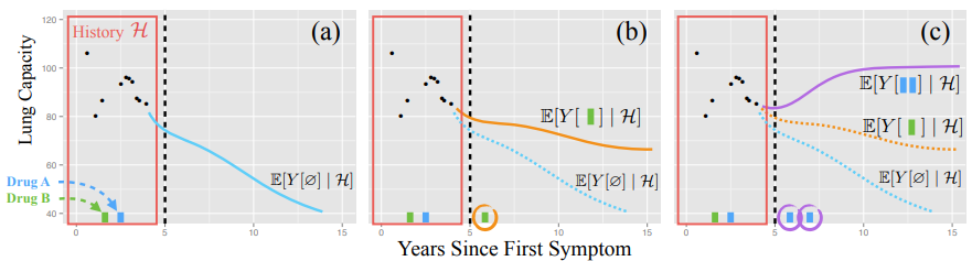
(a) : Evaluate risk if I do not intervene

검은색 점들은 이전의 lung capacity measurements이고 초록색과 파랑색 막대기는 treatment를 나타낸다.

파랑색 선은 no action일 때 일어나게 될 outcome에 대한 mean prediction이다.

(b), (c) : what if reasoning

Counterfactual trajectory under a single future green treatment

Counterfactual trajectory under two different action sequences

1.1 Contributions

우리의 핵심적인 method적인 기여는 CGP이다.

도출한 adjusted likelihood objective는 개인들의 observational trace $\mathcal{D}=\left\{\left\{\left(y_{i j}, a_{i j}, t_{i j}\right)\right\}_{j=1}^{n_{i}}\right\}_{i=1}^{m}$ 로부터 CGP를 학습하게 된다.

• CGP는 action을 선택하는데 사용한 policy의 outcome에 관한 effect를 제거한 predictor를 준다.
• CGP는 observed action과 outcome을 marked point process로 동시에 모델링하여 도출됐다.
• CGP는 counterfactual을 학습하는 데에 필요한 assumption들을 우리의 셋팅에 맞춰져서 도출됐다.

그리고 CGP를 활용하여 decision-support task를 수행하는 것을 보이도록 하겠다.

1.2 Related Work

Decision-support에 관한 이야기는 너무 넓고, 우리의 method적인 기여는 counterfactual model for time series이므로 method적인 부분만 이야기를 해보겠다.

Causal Inference

Counterfactual model은 action이 일어날 때와 안 일어날 때의 counterfactual outcome의 차이로 causal effect of action을 잰다.

보통, counterfactual을 formalize하고 causal effect를 estimate하는 데에선 potential outcome framework를 사용한다.

Potential outcomes in continuous time

Robins는 causal effect of a sequence of actions in discrete time on a final single outcome을 학습하기 위해서 potential outcomes framework을 확장하였다.

Arjas는 continuous time에서의 action들에 대해서 bayesian posterior predictive distribution으로 해결했다.

Lok와 Arjas and Parner는 continuous time observational data에서 CE of actions를 학습하기 위해서 marked point process를 사용하여 가정들을 formalize하였다.

우리는 MPP를 사용하여 continuous-time trajectories에 대한 causal effects of actions를 학습할 수 있다.

---

Treatment effects의 expressiveness를 고려한 최근의 논문들도 있다.

Xu는 모델의 flexibility를 위해서 BNP(DP, GP, …)를 제안하였고 그 외의 것들은 생략하도록 하겠다.

Reinforcement Learning

RL은 action과 observation이 discrete time에 배치된 데이터로부터 학습한다.

하지만 RL에선 model을 학습하기 보다는 expected reward를 최적화하는 policy를 학습하는 데에 집중한다.

Model-based RL에서 action effect의 모델은

1. policy를 최적화하기 전에 offline으로 생성되거나
2. agent가 그의 environment와 상호작용 하면서 점진적으로 생성된다.

대부분의 RL에서는 학습 알고리즘은 sample을 수집하기 위해 active experiment(시뮬레이션)에 의존하게 된다.

하지만 헬스케어에선 환자들을 actively experiment할 수 없기 때문에 obervational data에 의존해야만 한다.

RL에선 이를 off-policy evaluation으로 부른다.

Off-policy RL에선,

• unknown policy 하에서 agent에 의해 생성된 state-action-reward sequence를 사용하여
• target policy의 expected reward를 estimate 한다.

Off-policy algorithm은 일반적으로 expected reward를 학습하기 위해

1. action-value function의 approximation
2. importance-reweighting
3. 1+2

를 사용한다.

2. Counterfactual Models from Observational Traces

CGP는 potential outcomes와 Gaussian Process와 marked point processes로 부터 아이디어들을 가져왔다.

2.1 Background: Potential Outcomes

우리는 $\{Y[a]:a \in \mathcal{C}\}$를 모델링하려고 한다. 그래서 features $X$가 주어졌을 때 $P(Y[a] \mid X)$를 학습해야만 한다.

만약 자유롭게 action $a$을 input으로 넣고 $Y$를 기록할 수 있다면, 이는 단순한 모델 피팅 문제이다.

하지만, 이는 불가능하고 그저 $(A, Y, X)$에 관한 observational data만 사용할 수 있다.

일반적인 머신러닝에선, $P(Y \mid A, X)$를 모델링하고 observational data을 Supervised Learning algorithm으로 학습하게 된다.

여기서 만약 2개의 가정이 추가된다면, 제안한 conditional distribution을 counterfactual model으로 사용할 수 있다.

---

Assumption 1 (Consistency)

​ Let $Y$ be the observed outcome.

​ Let $A \in \mathcal C$ be the observed action.

​ Let $Y[a]$ be the potential outcome for action $a\in \mathcal C$.

​ Then,

$$(Y \triangleq Y[a]) \mid A=a$$

It implies that $P(Y \mid A=a)=P(Y[a] \mid A=a)$

Miguel Herman의 what if에선, treatment 버전의 다양성이 있으면 안된다고 언급하였다.

두번 째는 feature(covariate) $X$가 $Y[a]$와 $A$를 d-separate하는 데에 필요한 confounder들을 포함한다는 것이다.

---

Assumption 2 (No Unmeasured Confounders (NUC))

​ Let $Y$ be the observed outcome

​ Let $A \in \mathcal C$ be the observed action

​ Let $X$ be a vector containing all potential confounders.

​ Let $Y[a]$ be the potential outcome for action $a\in \mathcal C$.

​ Then, $(Y[a] \perp A) \mid X$

---

Assumption 1 and 2 implies $P(Y \mid A, X)=P(Y[a] \mid X)$

이의 sequence of actions 버전으로의 확장은 sequential NUC로 알려져있으나,
continuous time 셋팅에선 action의 타이밍이 potential outcomes에 statistically dependent하기 때문에 적용될 수 없다.

2.2 Background: Marked Point Processes

Point processes는 timestamps $\left\{T_{i}\right\}_{i=1}^{N}$ point들의 발생 위치에 대한 distribution이다.

Marked point processes는 point processes에 additional random variable $X_i$이 붙어있다.

예를 들어, 고객의 도착시간($T$)을 나타내는 process가 있다면 추가로 붙는 $X$는 그 고객이 상점에서 소비한 금액을 나타낼 수 있다.

Marked point processes는 다음의 random variables에 대한 분포를 나타낸다.

• the number of points $N$
• $(T_i, X_i)$

Point Process는 counting process $\left\{N_{t}: t \geq 0\right\}$로 완벽하게 characterized된다.

Counting process는 다음의 분포를 나타낸다.

• the number of points $N$
• $N_{t}=\sum_{i=1}^{N} \mathbb{I}_{\left(T_{i} \leq t\right)}$

Counting Process에 대한 일반적인 가정

1. $N_{t} \geq N_{s} \text { if } t \geq s$
2. $N_{0}=0$
3. $\Delta N_{t}=\lim _{\delta \rightarrow 0^{+}} N_{t}-N_{t-\delta} \in\{0,1\}$

Point process에 대한 parameterization은 history $\mathcal H_{t^-}$가 주어졌을 때 $\Delta N_{t}$에 대한 probabilistic model로 이루어질 수 있다.

Doob-Meyer decomposition을 사용하여, $\Delta N_{t}=\Delta M_{t}+\Delta \Lambda_{t}$으로 분해할 수 있다.

where $M_t$ is a martingale and $\Lambda_{t}$ is a cumulative intensity function.

$$\begin{aligned} P\left(\Delta N_{t}=1 \mid \mathcal{H}_{t^{-}}\right)&=\mathbb{E}\left[\Delta N_{t} \mid \mathcal{H}_{t^{-}}\right] \\ &=\mathbb{E}\left[\Delta M_{t} \mid \mathcal{H}_{t^{-}}\right]+\Delta \Lambda_{t}\left(\mathcal{H}_{t^{-}}\right) \\ &=0+\Delta \Lambda_{t}\left(\mathcal{H}_{t^{-}}\right) \end{aligned}$$

where $\lambda^{*}(t) \mathrm{d} t \triangleq \Delta \Lambda_{t}\left(\mathcal{H}_{t^{-}}\right)$

만약 $N_t$를 non-homogeneous Poisson-process를 사용한다면, intensity function은 history $H_{t^-}$에 의존하지 않는다.

반대로 MPP를 사용하면 $\lambda^{*}(t)$는 history에 의존한다.

---

이러한 Point Process로부터 정의된 MPP의 intensity function은 $\lambda^{}(t, x)=\lambda^{}(t) p^{*}(x \mid t)$으로 정의된다.

2.3 Counterfactual Gaussian Processes

2.3.1 Notation

Let $\left\{Y_{t}: t \in[0, \tau]\right\}$ denote a continuous-time stochastic process where

1. $Y_{t} \in \mathbb{R}$
2. $[0, \tau]$ defines the interval over which process is defined.

Let

1. the process is observed at a discrete set of irregular and random times $\left\{\left(y_{j}, t_{j}\right)\right\}_{j=1}^{n}$
2. $\mathcal C$ denote the set of possible action types
3. an action be a tuple $(a, t)$ where $a \in \mathcal C $ and $t \in [0, \tau]$
4. $\mathbf{a}=\left[\left(a_{1}, t_{1}\right), \ldots,\left(a_{n}, t_{n}\right)\right]$
5. $\mathcal{H}_{t}$ be a list of all previous observations of the process and all previous actions

---

Then, our goal is to model the counterfactual

$$P\left(\left\{Y_{s}[\mathbf{a}]: s>t\right\} \mid \mathcal{H}_{t}\right), \text { where } \mathbf{a}=\left\{\left(a_{j}, t_{j}\right): t_{j}>t\right\}_{j=1}^{n}$$

---

우리는 individual history $\mathbf h_i$들을 가지고서 학습을 할 것이다.

$$\mathbf{h}_{i}=\left\{\left(t_{i j}, y_{i j}, a_{i j}\right)\right\}_{j=1}^{n_{i}}$$

이들의 집합을 traces $\mathcal{D} \triangleq\left\{\mathbf{h}_{i}=\left\{\left(t_{i j}, y_{i j}, a_{i j}\right)\right\}_{j=1}^{n_{i}}\right\}_{i=1}^{m}$라고 하겠다.

where

1. $y_{i j} \in \mathbb{R} \cup\{\varnothing\}$
2. $a_{i j} \in \mathcal{C} \cup\{\varnothing\}$
3. $t_{i j} \in[0, \tau]$

우리의 방식은 traces $\mathcal{D}$를 MPP를 가지고서 모델링하는 것이다.

MPP의 state space는 $\mathbb{R} \times \mathcal{C}$처럼 보이지만 빈 값을 명시하는 indicator $z_{y} \in\{0,1\} \text { and } z_{a} \in\{0,1\}$를 추가하여

$$\mathcal{X}=(\mathbb{R} \cup\{\varnothing\}) \times(\mathcal{C} \cup\{\varnothing\}) \times\{0,1\} \times\{0,1\}$$

이 된다. 이 경우에 MPP의 intensity function은

$$\lambda^{*}\left(t, y, a, z_{y}, z_{a}\right)=\underbrace{\lambda^{*}(t) p^{*}\left(z_{y}, z_{a} \mid t\right)}_{\text {[A] Event model }} \underbrace{p^{*}\left(y \mid t, z_{y}\right)}_{\text {[B] Outcome model (GP) }} \underbrace{p^{*}\left(a \mid y, t, z_{a}\right)}_{\text {[C] Action model }}$$

$*$표시는 분포(또는 함수)가 history $\mathcal H_{t^-}$에 의존한다는 것을 강조하기 위함이다.

• Event model은 action의 빈도와 observation의 빈도를 의미한다.
• Action model은 과거에 기반한 action의 선택을 의미한다.
• 이 둘은 domain knowledge로 선택될 수 있다.
• Outcome model은 이전의 actions와 outcomes observation이 있을 때, 미래의 outcome을 GP로 예측하는 영역이다.

2.3.1 Learning

CGP를 학습하기 위해선, trace들이 서로 독립이라 가정할 경우에 sum of individual-trace log likelihood를 최대화 해야한다.

Let $\theta$ denote the model parameters, then the log likelihood for a single trace is

$$\ell(\boldsymbol{\theta})=\sum_{j=1}^{n} \log p_{\theta}^{*}\left(y_{j} \mid t_{j}, z_{y j}\right)+\sum_{j=1}^{n} \log \lambda_{\theta}^{*}\left(t_{j}\right) p_{\theta}^{*}\left(a_{j}, z_{y j}, z_{a j} \mid t_{j}, y_{j}\right)-\int_{0}^{\tau} \lambda_{\theta}^{*}(s) \mathrm{d} s$$

해석하자면, 첫번째 항은 GP를 outcome data에 피팅하는 역할이고 두번째 항은 $t, y, a$ 간의 dependency를 설명하는 역할이다.

2.3.2 Connection to target counterfactual

Learning objective를 maximize하면, observational traces $\mathcal D$의 statistical model을 얻게 된다.

일반적으로, statistical model은 target counterfactual을 모델링하는 것이 아니다.

$$p^{*}\left(y \mid t, z_{y}=1\right) = P\left(\left\{Y_{s}[\mathbf{a}]: s>t\right\} \mid \mathcal{H}_{t}\right)$$

를 위해선, assumption 2를 대신할 2가지의 추가 assumption이 필요하다.

Assumption 3 (Continuous-Time NUC)

​ For all times $t$ and all histories $\mathcal H_{t^{-}}$,

$$\text{densities $\lambda ^*(t), p^* (z_y, z_a \mid t), \text{ and } p^*(a \mid y, t, z_a)$ do not depend on $Y_{s}[\mathbf{a}]$}$$

직감적으로 해석하면, observational data에서 action을 선택하는데 사용한 policy와 future potential outcome가 독립이다.

Assumption 4 (Non-Informative Measurement Times)

​ For all times $t$ and any history $\mathcal{H}_{t^{-}}$, the following holds

$$p^{*}\left(y \mid t, z_{y}=1\right) \mathrm{d} y=P\left(Y_{t} \in \mathrm{d} y \mid \mathcal{H}_{t^{-}}\right)$$

펄의 causality에서 말하길 가정들은 통계적으로 검증이 불가능하다고 한다.

Proof

$$p^{*}\left(y \mid t, z_{y}=1\right) = P\left(\left\{Y_{s}[\mathbf{a}]: s>t\right\} \mid \mathcal{H}_{t}\right)$$

Notation부터 정리하자.

• $\mathbf q = [s_1, \ldots, s_m]$
  $t$ 시점 이후의 미래 계측이 이뤄지는 시점들
• $\mathbf a = [(t_1^\prime, a_1), …]$
  $t$ 시점 이후의 미래 action들
• $\mathbf O_i =\{ (s, Y_s, \emptyset, 1, 0) : s \in \mathbf q, s < s_i \}$
  $s_i$ 시점 이전에 일어난 계측 Event
• $\mathbf A_i =\{ (t^\prime, \emptyset, a, 0, 1) : (t^\prime, a) \in \mathbf a, s < s_i \}$
  $s_i$ 시점 이전에 일어난 action Event

$$\begin{aligned} P\left(\left\{Y_{s}[\mathbf{a}]: s \in \mathbf{q}\right\} \mid \mathcal{H}_{t}\right) &=\prod_{i=1}^{m} P\left(Y_{s_{i}}[\mathbf{a}] \mid\left\{Y_{s}[\mathbf{a}]: s \in \mathbf{q}, s<s_{i}\right\}, \mathcal{H}_{t}\right) \\ &= \prod_{i=1}^{m} P\left(Y_{s_{i}}[\mathbf{a}] \mid A_i,\left\{Y_{s}[\mathbf{a}]: s \in \mathbf{q}, s<s_{i}\right\}, \mathcal{H}_{t}\right) \\ &\quad \because \text{Assumption 3 $\approx$ Exchangeability} \\ &= \prod_{i=1}^{m} P\left(Y_{s_{i}} \mid A_i,\left\{Y_{s}: s \in \mathbf{q}, s<s_{i}\right\}, \mathcal{H}_{t}\right) \\ &\quad\because \text{Consistency} \\ &= \prod_{i=1}^{m} P\left(Y_{s_{i}} \mid A_i, O_i, \mathcal{H}_{t}\right) =: \prod_{i=1}^{m} P\left(Y_{s_{i}} \mid \mathcal{H}_{s_i}^-\right) \\ \prod_{i=1}^{m} P\left(Y_{s_{i}} \in dy \mid \mathcal{H}_{s_i}^-\right) &= \prod_{i=1}^{m} p^\star(y \mid s_i, z_y=1) dy \end{aligned}$$

3. Experiments

CGP를 2가지 의사결정보조 task에서 설명하겠다.

1. Training data에 존재하는 policy에 의존하지 않는 risk prediction
2. 개인의 치료계획을 위한 counterfactuals 비교

3.1 Reliable Risk Prediction with CGPs

계측 결과가 임계치 이하로 떨어질 가능성이 낮다면 귀가시키는 상황이다.

Policy $\pi_A, \pi_B$는 가정3을 지켰고, $\pi_C$는 이를 지키지 않아 가정의 유효함의 증명이 필수적이라는 것을 강조했다.

$\pi_A$는 테스트셋에서 사용하는 policy와 같다.

---

Simulation

계측 데이터는 3가지 GP의 mixture를 base로 생성했다.

• covariate function은 같음
• mean function은
  • 감소궤적
  • 유지궤적
  • 감소후 유지 궤적

Policy는 supplement에 설명

Treatment는 계측값을 2시간 후에 증가시킴

---

Model

• covariate function, mean fuction에 대한 정보 없이
• Outcome model에 3-mixture of GP를 사용

---

Comparison

• 일반 GP는 policy 변화에 취약하다.
• 반면에 CGP는 policy 변화에 robust하다.

3.2 “What if?” Reasoning for Individualized Treatment Planning

크레아티닌이 너무 높으면 신장에 문제가 생긴다.

3가지 치료가 있다. (IHD, CVVH, CVVHD)

셔플링을 하고 300명은 training data, 50명은 validation, 78명은 test로 쓴다.

---

Model

TE의 short-term + long-term을 모델링하기 위해 다음과 같이 mean ftn을 뒀다.

$$\begin{aligned} g\left(\delta ; h_{1}, a, b, h_{2}, r\right)&=g_{s}\left(\delta ; h_{1}, a, b\right)+g_{\ell}\left(\delta ; h_{2}, r\right) \\ &=\frac{h_{1} a}{a-b}\left(e^{-b \cdot t}-e^{-a \cdot t}\right) + h_2(1.0 - e^{-r\cdot t}) \end{aligned}$$

GP의 mixture 수는 validation set으로 결정됐다. (=3)

---

Results

• Test set에서 뽑힌 개인들을 나타낸다.
• 초록점 : 관측값 + posterior의 재료
• 빨간점 : 향후값
• 회색선 : 실제 행해진 treatment을 반영한 CGP의 mean function
• 파랑선 : 반사실적 treatment를 반영한 CGP의 mean function
• 회색구간 : MAP 기준 95% credible interval

Counterfactual에 대해선 계량적 평가가 불가능하다.

그저 baseline 모델과 비교해야한다.

Factual에 대해선 더 나은 성능을 보였다.