Recasting Gradient-Based Meta-Learning as Hierarchical Bayes

0. Abstract

Meta-learning(ML)은 agent가 이전의 episode를 기반으로 새로운 task에서 빠르게 적응하도록 한다.

Hierarchical Bayesian Model은 task들 간의 공유되는 parameter의 분포를 추론하는 문제로 ML을 formalize하는 이론적 framework를 제공한다.

우리는 MAML을 probabilistic inference in HBM으로 formalize한다.

기존의 HBM을 활용한 ML 방법들과 달리, MAML은 task-specific parameter의 posterior inference를 GD로 대체하기에 복잡한 함수로의 적용이 가능하다.

MAML을 HBM으로 받아들이면,

1. ML의 작동원리를 이해할 수 있고
2. Efficient inference의 기회를 제공한다.

1. Introduction

사람은 novel problem이 빠르게 해결할 수 있는 능력이 있다.

그러한 빠른 adaptation은 이전의 학습 경험을 활용함으로 이뤄진다.

ML의 meta-knowledge는 이전의 학습경험을 활용해서 AI agent가 제한된 data로 학습할 수 있음을 하게 해준다.

머신러닝에서, ML은 새로운 task에서의 학습의 효율을 향상시키는 inductive bias로 작동할 수 있는 domain-general information을 extract하여 formulate될 수 있다.

이 inductive bias는 다양하게 구현되어왔다.

1. HBM : Task-specific parameter를 제한하는 hyperparameter로서
2. Learned-Metric space : …
3. RNN의 weight을 meta-knowledge로 활용하여 hidden-state를 활용함으로서
4. Optimization algorithm의 parameter로서

---

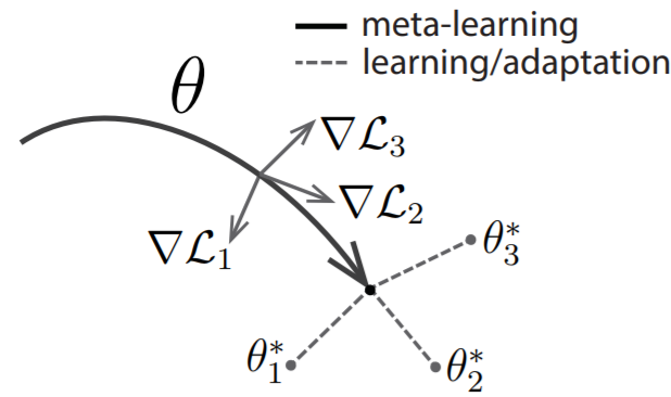
MAML은 4에 속하며, model의 initial parameter를 fast adaptation을 위한 inductive bias로 활용하였다.

MAML의 inductive bias는 empirically evaluate되어왔다.

---

이 논문에선, MAML을,
HBM에서의 task들 간에 공유하는 parameter의 prior distribution을 추론하는 문제로 이해됨을 보인다.

MAML의 학습된 prior는 implicit predictive distribution over task-specific parameter에 기반하여 빠르게 unseen task에 adapt한다.

MAML을 HBM으로 해석하게 되면, bayesian posterior estimation으로 부터 insight를 가져와서, MAML을 향상시킬 수 있게 된다.

2. Meta-Learning Formulation

Meta-learner의 목표는 다양한 task의 경험을 통해 task-general knowledge를 extract하는 것이다.

이를 prior knowledge로 활용하여, learner는 새로운 task에 빠르게 adapt할 수 있다.

Task들이 common structure를 공유하기 때문에 한 task의 학습이 다른 task의 학습에 도움이 될 수 있다.

Meta-learner의 objective function은 $\mathcal T \sim p(\mathcal T)$에서의 task-specific performance를 최대화하는 것이다.

---

ML을 2가지 방법으로 formulate하겠다.

1. gradient-based hyperparameter optimization
2. probabilistic inference in HBM

이들은 따로 발전되어왔지만, 3.1에서 이들을 엮어보겠다.

2.1 Meta-Learning as Gradient-Based Hyperparameter Optimization

Parametric meta-learner는 novel task를 만났을 때, 이에 맞는 task-specific parameter $\boldsymbol \phi$를 찾는걸 쉽게해주는 $\boldsymbol \theta$를 찾는 걸 도와준다.

Gradient method들을 사용하는 이전의 방법들과 달리 MAML은 $\boldsymbol \phi$와 $\boldsymbol \theta$가 같은 space에 있는 방법이다.

$$\mathcal{L}(\boldsymbol{\theta})=\frac{1}{J} \sum_{j}\left[\frac{1}{M} \sum_{m}-\log p(\mathbf{x}_{j_{N+m}} \mid \underbrace{\boldsymbol{\theta}-\alpha \nabla_{\boldsymbol{\theta}} \frac{1}{N} \sum_{n}-\log p\left(\mathbf{x}_{j_{n}} \mid \boldsymbol{\theta}\right)}_{\boldsymbol{\phi}_{j}})\right]$$

where $\boldsymbol \phi_{j}$ is the updated task-specific parameter

2.2 Meta-Learning as Hierarchical Bayesian Inference

메타러닝을 HBM에서의 probabilistic inference로 볼 수도 있다.

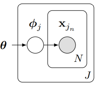
메타러닝에서, task-specific parameter $\boldsymbol \phi _j$는 구분되었지만 이의 estimation이 $\left\{\boldsymbol \phi_{j^{\prime}} \mid j^{\prime} \neq j\right\}$ estimation에 영향을 줘야한다.

이를 위해 meta-level parameter $\boldsymbol \theta$를 도입하게 된다.

이 구조에서 $\boldsymbol \theta$에 대한 estimate은 $\boldsymbol \phi_j$의 inference에 제한을 주게된다.

$$p(\mathbf{X} \mid \boldsymbol{\theta})=\prod_{j}\left(\int p\left(\mathbf{x}_{j_{1}}, \ldots, \mathbf{x}_{j_{N}} \mid \boldsymbol \phi_{j}\right) p\left(\boldsymbol \phi_{j} \mid \boldsymbol{\theta}\right) \mathrm{d} \boldsymbol{\phi}_{j}\right)$$

이를 maximizing하는 것은 empirical Bayes라고 알려졌다.

Prior distribution의 parameter $\theta$를 estimate하는 데에 data를 사용했다는 관점에서

HBM은 transfer learning과 domain adaptation에서 사용의 역사가 있다.

하지만 HBM은 inference procedure를 제공하지 않고 복잡한 모델에 대해서 tractability를 제공하지 않는다.

3. Linking Gradient-Based Meta-Learning & Hierarchical Bayes

MAML이 empirical Bayes in HBM로 이해될 수 있음을 보여서, 위의 둘을 연결짓겠다.

MAML의 meta-learning은 Task-specific prior distribution $p\left(\boldsymbol{\phi}_{j} \mid \boldsymbol{\theta}\right)$을 선택하는 과정이다.

3.1 MAML as Empirical Bayes

일반적으로 marginalization over task-specific parameters $\boldsymbol \phi_j$은 tractable하지 않다.

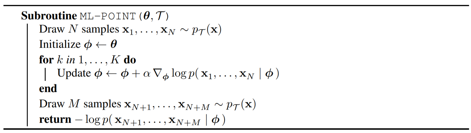
대안으로, point estimate $\hat {\boldsymbol \phi_j}$으로 대체하는 것이다.

$$\begin{aligned} p(\mathbf{X} \mid \boldsymbol{\theta}) &=\prod_{j}\left(\int p\left(\mathbf{x}_{j_{1}}, \ldots, \mathbf{x}_{j_{N}} \mid \boldsymbol \phi_{j}\right) p\left(\boldsymbol \phi_{j} \mid \boldsymbol{\theta}\right) \mathrm{d} \boldsymbol{\phi}_{j}\right) \\ &\approx \prod_{j} p\left(\mathbf{x}_{j_{1}}, \ldots, \mathbf{x}_{j_{N}} \mid \hat{\boldsymbol \phi_{j}}\right) \\ \\ -\log p(\mathbf{X} \mid \boldsymbol{\theta}) & \approx \sum_{j}\left[-\log p\left(\mathbf{x}_{j_{N+1}}, \ldots \mathbf{x}_{j_{N+M}} \mid \hat{\boldsymbol{\phi}}_{j}\right)\right] \end{aligned}$$

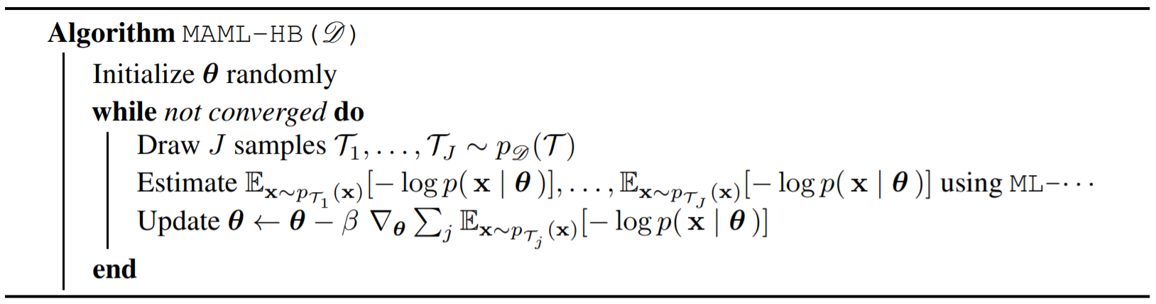
$\hat{\boldsymbol{\phi}}_{j}=\boldsymbol{\theta}+\alpha \nabla_{\boldsymbol{\theta}} \log p\left(\mathbf{x}_{j_{1}}, \ldots, \mathbf{x}_{j_{N}} \mid \boldsymbol{\theta}\right)$로 두게 되면 이는 one-step MAML의 objective가 된다.

$\hat{\boldsymbol{\phi}}_{j}$는 $\boldsymbol \theta$에서 크게 벗어나지 않는 선에서, $-\log p(\mathbf{X} \mid \boldsymbol{\theta}) $를 줄이는 것에 대응된다.

---

Linear regression case에서 이러한 trade-off를 HBM으로 formalize할 수 있다.

Linear model에서 early stopping of GD의 옵션은 특정 prior(step의 횟수 direction에 의존하는) 하에서 MAP를 구하는 것이다.

$$\begin{aligned} \boldsymbol{\phi}_{(k)} &=\boldsymbol{\phi}_{(k-1)}-\alpha \nabla_{\boldsymbol{\phi}}\left[\|\mathbf{y}-\mathbf{X} \boldsymbol{\phi}\|_{2}^{2}\right]_{\phi=\boldsymbol{\phi}_{(k-1)}} \\ &=\boldsymbol \phi_{(k-1)}-\alpha \mathbf{X}^{\mathrm{T}}\left(\mathbf{X} \boldsymbol \phi_{(k-1)}-\mathbf{y}\right) \end{aligned}$$

Santos, 1996은 $\boldsymbol \phi_{(0)}=\boldsymbol \theta$에서 시작하는 것은 $\min \left(|\mathbf{y}-\mathbf{X} \boldsymbol{\phi}|_{2}^{2}+|\boldsymbol{\theta}-\boldsymbol{\phi}|_{\mathbf{Q}}^{2}\right)$를 최적화하는 것이라고 했다.

이 부분은 수식이 애매하게 넘어감.

$\min \left(|\mathbf{y}-\mathbf{X} \boldsymbol{\phi}|_{2}^{2}+|\boldsymbol{\theta}-\boldsymbol{\phi}|_{\mathbf{Q}}^{2}\right)$는 MAP를 구하는 것에 대응된다.

• $\boldsymbol \phi \sim \mathcal{N}(\boldsymbol \phi ; \boldsymbol{\theta}, \mathbf{Q})$
• $ \mathbf y \mid \mathbf X, \boldsymbol \phi \sim \mathcal{N}(\mathbf{y} ; \mathbf{X} \boldsymbol \phi, \mathbb{I})$

그러므로 Linear regression에서의 MAML은 implicit prior하에서 empirical Bayes를 하는 것에 대응된다.

---

Nonlinear의 경우엔, MAML은 empirical Bayes procedure와 동일하지만 $\boldsymbol \phi$가 MAP에 대응되진 않는다.

그 뒤에 뭐라 말을 했는데 그런가보다 하고 넘어감

MAP 대신에 implicit MAP라는 표현을 사용함

결국 MAML은 MAP로 marginal likelihood를 approximate하고 난 뒤에 $\boldsymbol \theta$를 update하는 것이다.

$$\mathbb{E}_{\mathbf{x} \sim p_{\mathcal{T}_{j}}(\mathbf{x})}[-\log p(\mathbf{x} \mid \boldsymbol{\theta})] \approx \frac{1}{M} \sum_{m}-\log p\left(\mathbf{x}_{j_{N+m}} \mid \hat{\boldsymbol{\phi}}_{j}\right)$$

---

3.2 The Prior over Task-Specific Parameters

3.1에서 early stopping(fast adaptation)은 prior selection과 동일하다고 결론지었다.

Let $\phi^\star$ be a minima of fast adaptation objective $\ell(\phi)=-\log p\left(\mathbf{x}_{1} \ldots, \mathbf{x}_{N} \mid \phi\right)$

Consider second-order approximation

$$\ell(\boldsymbol\phi) \approx \tilde{\ell}(\boldsymbol\phi):=\frac{1}{2}\left\|\boldsymbol\phi-\boldsymbol\phi^{*}\right\|_{\mathbf{H}^{-1}}^{2}+\ell\left(\boldsymbol\phi^{*}\right)$$

where $\mathbf{H}=\nabla_{\boldsymbol{\phi}}^{2} \ell\left(\boldsymbol{\phi}^{*}\right)$ is assumed to be positive definite.

Consider the gradient descent with curvature matrix $\mathcal B$

$$\boldsymbol\phi_{(k)}=\boldsymbol\phi_{(k-1)}-\mathcal{B} \nabla_{\boldsymbol\phi} \tilde{\ell}\left(\boldsymbol\phi_{(k-1)}\right)$$

If $\mathcal B$ is diagonal, then the update corresponds to a Newton method with a diagonal approximation.

Meta-learned matrix $\mathcal B$는 fast adaptation prior $p(\boldsymbol \phi \mid \boldsymbol \theta)$의 covariance matrix에 task-general information을 담는 것이다.

위의 GD는 w/ $\boldsymbol \phi_{(0)} = \boldsymbol \theta$

$$\min \left(\left\|\boldsymbol \phi-\boldsymbol\phi^{*}\right\|_{\mathbf{H}^{-1}}^{2}+\left\|\boldsymbol\theta -\boldsymbol\phi\right\|_{\mathbf{Q}}^{2}\right)$$

을 푸는 것이다.

• $\boldsymbol \phi \sim \mathcal{N}(\boldsymbol \phi ; \boldsymbol{\theta}, \mathbf{Q})$

  • $\mathbf{Q}=…$

    잘 모르겠음 이해하려면 Santos 1996 읽어야 할 듯

• $\left|\boldsymbol \phi-\boldsymbol\phi^{*}\right|_{\mathbf{H}^{-1}}^{2}$는 뭐에 대응하는 것 인지 언급없음

4. Improving MAML

MAML을 HBM의 empirical Bayes로 받아들이면 이를 발전시킬 수 있다.

4.1 Laplace’s Method of Integration

MAML은 empirical Bayes w/ point estimate task-specific parameter in HBM이다.

그러나, point estimate의 사용은 부정확한 approximate이 될 수 있다.

$$-\log p(\mathbf{X} \mid \boldsymbol{\theta}) \approx \sum_{j}\left[-\log p\left(\mathbf{x}_{j_{N+1}}, \ldots \mathbf{x}_{j_{N+M}} \mid \hat{\boldsymbol{\phi}}_{j}\right)\right]$$

특히, posterior $\boldsymbol \phi$가 그렇게 sharp하지 않을 수록.

Laplace approximation은 이 경우에 적용이 가능하다.

---

Suppose function $f(x)$ has a unique global maximum at $x_0$

Let $M$ be a constant and consider the following two eqns

• $g(x)=M f(x)$
  • $\frac{g\left(x_{0}\right)}{g(x)}=\frac{M f\left(x_{0}\right)}{M f(x)}=\frac{f\left(x_{0}\right)}{f(x)}$
• $h(x)=e^{M f(x)}$
  • $\frac{h\left(x_{0}\right)}{h(x)}=\frac{e^{M f\left(x_{0}\right)}}{e^{M f(x)}}=e^{M\left(f\left(x_{0}\right)-f(x)\right)}$

As $M$ increases, the ratio for $h$ will grow exponentially, but not $g$

즉, $h$의 적분은 거의 $x_0$의 neighborhood에서 온다.

$$f(x)=f\left(x_{0}\right)+f^{\prime}\left(x_{0}\right)\left(x-x_{0}\right)+\frac{1}{2} f^{\prime \prime}\left(x_{0}\right)\left(x-x_{0}\right)^{2}+R \\ f(x) \approx f\left(x_{0}\right)-\frac{1}{2}\left|f^{\prime \prime}\left(x_{0}\right)\right|\left(x-x_{0}\right)^{2} \quad \text{for close $x$ to $x_0$}$$ $$\begin{aligned} \int_{a}^{b} e^{M f(x)} d x &= e^{M f\left(x_{0}\right)} \int_{a}^{b} e^{-\frac{1}{2} M\left|f^{\prime \prime}\left(x_{0}\right)\right|\left(x-x_{0}\right)^{2}} d x \quad \text{as $M \rightarrow \infty$} \\ &= \sqrt{\frac{2 \pi}{M\left|f^{\prime \prime}\left(x_{0}\right)\right|}} e^{M f\left(x_{0}\right)} \quad \because \text{Gaussian normalization} \end{aligned}$$

---

이 근사를 task-specific parameter에 적용할 경우,

$$\begin{aligned} \int p\left(\mathbf{X}_{j} \mid \boldsymbol{\phi}_{j}\right) p\left(\boldsymbol{\phi}_{j} \mid \boldsymbol{\theta}\right) \mathrm{d} \boldsymbol{\phi}_{j} & = \int \exp \left(\log p\left(\mathbf{X}_{j} \mid \boldsymbol{\phi}_{j}\right) + \log p\left(\boldsymbol{\phi}_{j} \mid \boldsymbol{\theta}\right)\right) \mathrm{d} \boldsymbol{\phi}_{j} \\ &= \int \exp \left(\log p\left(\boldsymbol{\phi}_{j} \mid \mathbf X_j , \boldsymbol{\theta}\right)\right) \mathrm{d} \boldsymbol{\phi}_{j} + C(\theta) \\ &\approx p\left(\mathbf{X}_{j} \mid \boldsymbol{\phi}_{j}^{*}\right) p\left(\boldsymbol{\phi}_{j}^{*} \mid \boldsymbol{\theta}\right) \operatorname{det}\left(\mathbf{H}_{j} / 2 \pi\right)^{-\frac{1}{2}} \end{aligned}$$

where $\mathbf{H}_{j}$ is the Hessian matrix of second derivatives of posterior.

Then, fast adaptation objective will be

$$-\log p(\mathbf{X} \mid \boldsymbol{\theta}) \approx \sum_{j}\left[-\log p\left(\mathbf{X}_{j} \mid \hat{\boldsymbol{\phi}}_{j}\right)-\log p\left(\hat{\boldsymbol{\phi}}_{j} \mid \boldsymbol{\theta}\right)+\frac{1}{2} \log \operatorname{det}\left(\mathbf{H}_{j}\right)\right]$$

Laplace approximation을 하게 되면 model의 complexity를 penalize하는 term $\frac{1}{2} \log \operatorname{det}\left(\mathbf{H}_{j}\right)$이 추가된다.

4.2 Using Curvature Information to Improve

Early stopping을 대변하는 prior $p(\boldsymbol \phi \mid \boldsymbol \theta)$가 implicit하기에 구할 수 있는 대상이 아니다.

그래서 그냥 간단한 Gaussian with $\tau$ precision으로 대체한다.

Hessian의 determinant 계산의 efficiency를 위해 Kronecker-factored approximate curvature (K-FAC)으로 대체한다.