Near-optimal Regret Bounds for Reinforcement Learning

0. Abstract

Undiscounted RL in MDP에서, total regret w.r.t. optimal policy를 고려한다.

MDP의 transition structure를 설명하기 위해서 특정 state까지 도달하는데 걸리는 step을 의미하는 diameter $D$를 도입한다.

임의의 MDP w/ $D$, $\mathcal S$, $\mathcal A$에 대해, total regret $\tilde{O}(D S \sqrt{A T})$을 만족하는 RL algorithm을 제시한다.

읽은 이유는 near optimal DTR의 증명을 이해하기 위해서이다.
아직 다 읽진 못했지만 나머지는 곧 읽을 것이다.

1. Introduction

MDP의 reward의 범위를 $\left [0, 1\right]$로 두겠다.

특정 알고리즘으로 학습된 policy의 performance보단, 학습 동안의 performance에 관심이 있다.

이를 위해, 몇가지 정의를 하자면

• Accumulated reward of algorithm $\mathfrak A$ after $T$ steps in MDP $M$ with initial state $s$
  • $R(M, \mathfrak{A}, s, T):=\sum_{t=1}^{T} r_{t}$
• Expected average reward of the process $(M, \mathfrak A, s)$
  • $\boldsymbol{\rho}(M, \mathfrak{A}, s):=\lim _{T \rightarrow \infty} \frac{1}{T} \mathbb{E}[R(M, \mathfrak{A}, s, T)]$

---

편의를 위해, stationary policy만 고려하겠다.

Optimal policy 학습의 어려움은 $| S|, |A|$ 뿐만 아니라 transition structure에도 의존한다.

Definition 1

​ Consider the stochastic process $(M, \pi , s)$

​ Let $T\left(s^{\prime} \mid M, \pi, s\right)$ be the random variable for the first time step w/ $s \Rightarrow s^\prime$

​ Then, the diameter of $M$ is defined as

$$D(M):=\max _{s \neq s^{\prime} \in S} \min _{\pi: S \rightarrow \mathcal{A}} \mathbb{E}\left[T\left(s^{\prime} \mid M, \pi, s\right)\right]$$

---

어떤 policy를 가져와도 특정 state에 도달하기 어렵다면 diameter는 커지게된다.

당연히 알고리즘의 regret의 bound는 finite diameter를 요구할 것처럼 보인다.

왜냐면 learner의 suboptimal action으로 explore한다면, 좋은 쪽으로 가는데 $D$ step이 걸리기 때문이다.

훨씬 간단한 MAB 문제에서 UCB 알고리즘이 $\sum \frac{\log T}{\text{gap}}$의 바운드를 갖기 때문에 $\Theta(D|S||\mathcal{A}| \log T)$ 일것이라고 기대할 수도 있다.

Mannor, 2004의 gap independent algorithm의 $\Omega(\sqrt{|\mathcal{B}| T})$를 생각해보면 $\Theta(\sqrt{D|S||\mathcal{A}| T})$ 일 것이라고 기대할 수도 있다.

Finite diameter를 갖는 경우에 optimal expected average reward는 initial state $s$에 의존하지 않는다.

$$\rho^{*}(M):=\rho^{*}(M, s):=\max _{\pi} \rho(M, \pi, s)$$

학습 알고리즘 $\mathfrak A$의 평가를 위해 total regret을 정의하자.

$$\Delta(M, \mathfrak{A}, s, T):=T \rho^{*}(M)-R(M, \mathfrak{A}, s, T)$$

우리가 제안할 UCRL2는 $\tilde{O}(D|\mathcal{S}| \sqrt{|\mathcal{A}| T})$의 total regret을 갖는다.

3. The UCRL2 Algorithm

UCRL Auer and Ortner, 2007처럼, UCRL2는 optimism in the face of uncertainty를 따른다.

• 이제까지의 observation들을 갖고서 statistically plausible MDP들의 집합 $\mathcal{M}$을 정의한다.
• Optimistic MDP $\tilde M \in \mathcal M$ w.r.t. optimal reward를 고른다.
• (nearly) optimal policy $\tilde{\pi}$ for $\tilde M$을 찾고 실행한다.

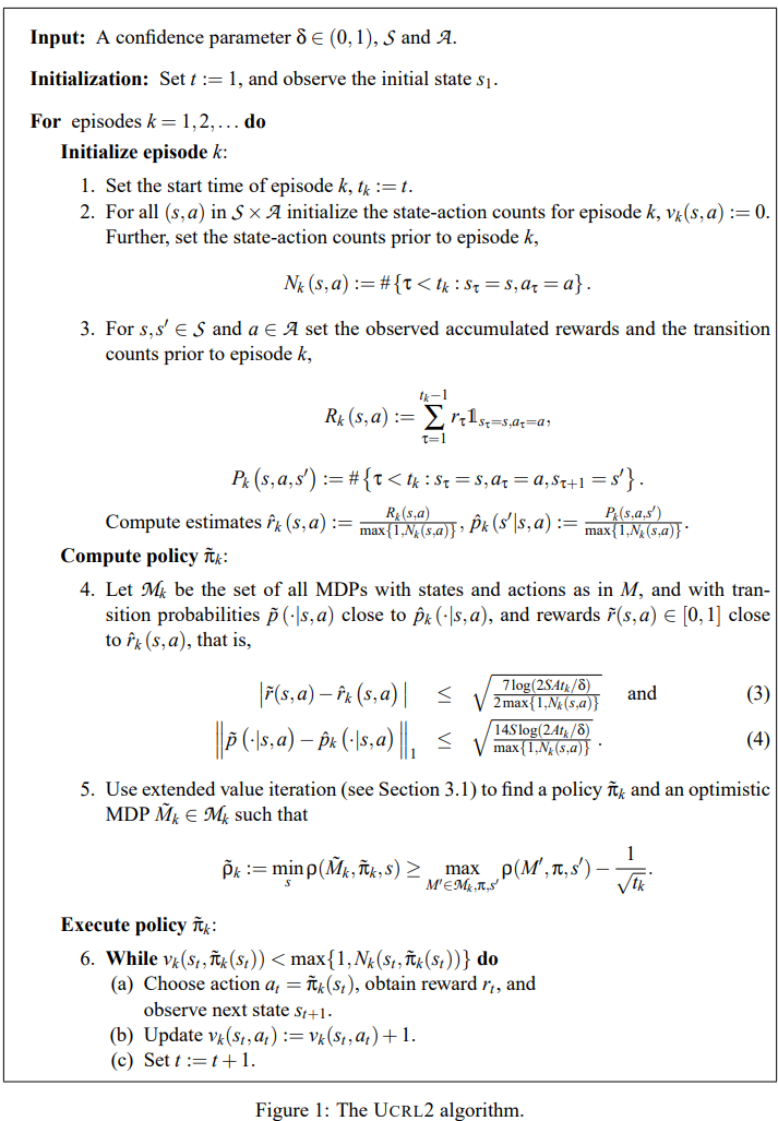
• Step 2+3 : empirically estimates $\hat{r}_{k}(s, a)$ and $\hat{p}_{k}\left(s^{\prime} \mid s, a\right)$
• Step 4 : 높은 확률로 true MDP $M$이 속해있는 plausible MDPs set $\mathcal M_k$ 정의
• Step 5 : extended value iteration to find near optimal $\tilde \pi_k$ and optimistic MDP $\tilde M_k \in \mathcal M_k$
• Step 6 : $\tilde \pi_k$를 실행하고 $(s_t, \tilde \pi_k(s_t))$가 $k$ episode 이전에 등장한 횟수를 넘기면 끝낸다.

3.1 Extended Value Iteration: Finding Optimistic Model and Optimal Policy

UCRL2에서 near optimal policy $\tilde \pi_k$와 optimistic MDP $\tilde M_k \in \mathcal M_k$를 찾을 필요가 있다.

일반적으로 VI는 fixed MDP에서 optimal policy를 찾아주지만, 우리는 plausible MDP 사이에서 가장 높은 average reward를 줄 MDP를 고를 필요가 있다.

3.1.1 Problem Formulation

Given $\hat p, \hat r$, let $\mathcal M$ be the set of all MDPs w/ $\tilde p$ and $\tilde r$ s.t.

$$\begin{aligned} \|\tilde{p}(\cdot \mid s, a)-\hat{p}(\cdot \mid s, a)\|_{1} & \leq d(s, a) \\ |\tilde{r}(s, a)-\hat{r}(s, a)| & \leq d^{\prime}(s, a) \end{aligned} \quad \text{where $r \in [0, 1]$}$$

UCRL2의 EVI에 사용되는 $d$와 $d^\prime$은 Step 4에서 정의한 confidence interval이다.

Assume

1. $M$ contains at least one MDP w/ finite diameter
2. True MDP has finite diameter

목표는 $\tilde \pi, \tilde M = \arg \max _{\pi , M \in \mathcal M} \rho\left(M^{\prime}, \pi, s^{\prime}\right)$를 찾는 것이다.

continuous action space 이야기를 꺼내는 데 왜 꺼내는 지 이해 안되니 일단 생략

3.1.2 Extended Value Iteration

Let $u_i(s)$ denote the state values of $i$-th iteration.

Then, undiscounted value iteration

$$\begin{aligned} u_{0}(s) &=0 \\ u_{i+1}(s) &=\max _{a \in \mathcal{A}}\left\{\tilde{r}(s, a)+\max _{p(\cdot) \in \mathcal{P}(s, a)}\left\{\sum_{s^{\prime} \in \mathcal{S}} p\left(s^{\prime}\right) \cdot u_{i}\left(s^{\prime}\right)\right\}\right\} \end{aligned}$$

Inner maximization은 linear optimization problem over the convex polytope $\mathcal{P}(s, a)$로 풀린다.

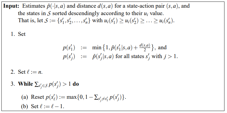
이 아이디어는

• state의 value가 낮은 쪽의 확률을 최대 $\frac{d(s,a)}{2}$만큼 끌어와서
• 가장 높은 쪽으로 transition probability를 할당하는 것이다.

3.1.3 Convergence of Extended Value Iteration

continuous action space 이야기를 꺼내는 데 왜 꺼내는 지 이해 안되니 일단 생략

Convergence를 보장하기 위해 EVI가 periodic transition matrix를 갖는 policy를 고르지 않음을 보이면 된다.

See Appendix B

사실 EVI는 $s_1^\prime$에 몰아주는 방식이기에 aperiodic transition matrix를 갖는 policy만 고른다.

Policy가 aperiodic이기에 state independent average reward를 갖는다.

Theorem 7

​ Let $\mathcal M$ be the set of MDPs.

​ If $\mathcal M$ contains at least one communicating MDP, stopping EVI when

$$\max _{s \in S}\left\{u_{i+1}(s)-u_{i}(s)\right\}-\min _{s \in S}\left\{u_{i+1}(s)-u_{i}(s)\right\}<\varepsilon$$

, the greedy policy w.r.t. $\mathbf u_i$ is $\epsilon$-optimal policy.

---

UCRL2의 step5는 $\epsilon = \frac{1}{\sqrt{t_{k}}}$에 대응한다.

$$\max _{s \in S}\left\{u_{i+1}(s)-u_{i}(s)\right\}-\min _{s \in S}\left\{u_{i+1}(s)-u_{i}(s)\right\}<\frac{1}{\sqrt{t_{k}}}$$

---

Remark 8

​ 나중에

4. Analysis of UCRL2

Let $\Delta_{k}:=\sum_{s, a} v_{k}(s, a)\left(\rho^{*}-\bar{r}(s, a)\right)$ be the regret in episode $k$

4.1에선 total regret이 episode 단위의 regret으로 나눠질 수 있음을 보인다.

4.2에선 true MDP를 포함하지 못한 episode들의 regret의 sum이 $\sqrt{T}$로 bound됨을 보인다.

4.3에선 true MDP를 포함한 episode의 regret의 bound를 보이겠다.

$$\Delta_{k} \leq \boldsymbol{v}_{k}\left(\tilde{\boldsymbol{P}}_{k}-\boldsymbol{I}\right) \boldsymbol{w}_{k}+2 \sum_{s, a} v_{k}(s, a) \sqrt{\frac{7 \log \left(2 S A t_{k} / \delta\right)}{2 \max \left\{1, N_{k}(s, a)\right\}}}+2 \sum_{s, a} \frac{v_{k}(s, a)}{\sqrt{t_{k}}}$$

4.4와 4.5에선 이 결과들을 묶어서 Theorem2와 Corollary3을 증명하겠다.

---

Theorem 2

$${}^\forall \text{initial state } s \in \mathcal S \text{ and } {}^\forall T >0, \\ \quad \Delta(M, \operatorname{UCRL2}, s, T) \leq 34 \cdot D S \sqrt{A T \log \left(\frac{T}{\delta}\right)} \quad \text{w/ pbt at least $1-\delta$}$$

---

Corollary 3

$$\text{Given } \epsilon > 0 \text{, } {}^\forall T \geq 4 \cdot 34^{2} \cdot \frac{D^{2} S^{2} A}{\varepsilon^{2}} \log \left(\frac{34 D S A}{\delta \varepsilon}\right), \\ \quad \frac{\Delta(M, \operatorname{UCRL2}, s, T) }{T} \leq \epsilon \quad \text{w/ pbt at least $1-\delta$}$$

4.1 Splitting into Episodes

Total regret을 episode 단위로 쪼개보자.

모든 (state, action) pair를 conditional로 뒀을 때, reward끼리 상호독립이므로 Hoeffding’s inequality를 적용하면

$$\begin{aligned} \mathbb{P}&\left\{\sum_{t=1}^{T} r_{t} \leq \sum_{s, a} N(s, a) \bar{r}(s, a)-\sqrt{\frac{5}{8} T \log \left(\frac{8 T}{\delta}\right)} \mid(N(s, a))_{s, a}\right\} \\ &\leq \exp(-2 \times \frac{5}{8} \log \frac{8T}{\delta}) = \left(\frac{\delta}{8 T}\right)^{5 / 4} \\ &<\frac{\delta}{12 T^{5 / 4}} \end{aligned}$$

이를 이용해 UCRL2의 total regret의 bound를 구할 수 있다.

$$\begin{aligned} \Delta\left(s_{1}, T\right)&=T \rho^{*}-\sum_{t=1}^{T} r_{t} \\ &<T \rho^{*}-\sum_{s, a} N(s, a) \bar{r}(s, a)+\sqrt{\frac{5}{8} T \log \left(\frac{8 T}{\delta}\right)} \quad \text{w/ pbt at least $1-\frac{\delta}{12 T^{5 / 4}}$} \end{aligned}$$

이제 이를 episode 단위로 나누기 위해 몇가지 notation을 도입하자면

• $m$ denotes the number of episodes up to $T$
• $\sum_{k=1}^{m} v_{k}(s, a)=N(s, a)$
• $\Delta_{k}:=\sum_{s, a} v_{k}(s, a)\left(\rho^{*}- \bar{r}(s, a)\right)$
• $\Delta_{k}$는UCRL2의 $k$번째 episode의 regret이다.

관계식을 이용하면 episode 단위로 나눠서 total regret의 bound를 구할 수 있다.

$$\Delta\left(s_{1}, T\right) \leq \sum_{k=1}^{m} \Delta_{k}+\sqrt{\frac{5}{8} T \log \left(\frac{8 T}{\delta}\right)} \quad \text{w/ pbt at least $1-\frac{\delta}{12 T^{5 / 4}}$}$$

4.2 Dealing with Failing Confidence Regions

True MDP를 포함하지 않는 episode들의 regret의 sum $\sum_{k=1}^{m} \Delta_{k} \mathbb{1}_{M \notin \mathcal{M}_{k}}$을 고려해보자.

Episode의 종료 조건에 의해 $v_{k}(s, a)=1 \text{ and } N_{k}(s, a)=0 \text{ and } \sum_{s, a} v_{k}(s, a)=1$인 trivial episode를 제외하곤,

$$\sum_{s, a} v_{k}(s, a) \leq \sum_{s, a} N_{k}(s, a)=t_{k}-1$$

Therefore,

$$\begin{aligned} \sum_{k=1}^{m} \Delta_{k} \mathbb{1}_{M \notin \mathcal{M}_{k}} &= \sum_{k=1}^{m} \left(\sum_{s, a} v_{k}(s, a)\left(\rho^{*}- \bar{r}(s, a)\right) \right )\mathbb{1}_{M \notin \mathcal{M}_{k}} \\ &\leq \sum_{k=1}^{m} \left(\sum_{s, a} v_{k}(s, a) \right )\mathbb{1}_{M \notin \mathcal{M}_{k}} \\ &\leq \sum_{k=1}^{m} t_k\mathbb{1}_{M \notin \mathcal{M}_{k}} = \sum_{t=1}^{T} t \sum_{k=1}^{m} \mathbb{1}_{t_{k}=t, M \notin \mathcal{M}_{k}} \\ &\leq \sum_{t=1}^{T} t \mathbb{1}_{M \notin \mathcal{M}(t)} \quad \text{where $\mathcal M(t) = \mathcal M_k$ w/ $t_k\leq t < t_{k+1}$} \\ &= \sum_{t=1}^{\left\lfloor T^{1 / 4}\right\rfloor} t \mathbb{1}_{M \notin \mathcal{M}(t)}+\sum_{t=\left\lfloor T^{1 / 4}\right\rfloor+1}^{T} t \mathbb{1}_{M \notin \mathcal{M}(t)} \\ &\leq \sqrt{T}+\sum_{t=\left\lfloor T^{1 / 4}\right\rfloor+1}^{T} t \mathbb{1}_{M \notin \mathcal{M}(t)} \end{aligned}$$

Furthermore, $\mathbb{P}\{M \notin \mathcal{M}(t)\} \leq \frac{\delta}{15 t^{6}}$ (see Appendix C.1)

Hence,

$$\begin{aligned} \mathbb P \left( \sum_{k=1}^{m} \Delta_{k} \mathbb{1}_{M \notin \mathcal{M}_{k}} \leq \sqrt T\right) &\geq \mathbb P \left( \sum_{t=\left\lfloor T^{1 / 4}\right\rfloor+1}^{T} t \mathbb{1}_{M \notin \mathcal{M}(t)} = 0\right) \\ &= 1- \mathbb P \left( \sum_{t=\left\lfloor T^{1 / 4}\right\rfloor+1}^{T} t \mathbb{1}_{M \notin \mathcal{M}(t)} \neq 0\right) \\ &= 1 - \mathbb P \left({}^{\exists}t \in (T^{1/4}, T] : \quad M \notin \mathcal{M}(t)\right) \\ &\geq 1- \sum_{t=1} ^T\mathbb P\left( M \notin \mathcal{M}(t)\right) \\ &\geq 1 - \sum_{t=1} ^T\frac{\delta}{15 t^{6}} \quad \because \text{see Appendix C.1} \\ &\geq 1 - \frac{\delta}{12 T^{5 / 4}} \end{aligned}$$

즉, true MDP를 포함하지 못한 episode들의 regret의 sum이 $\sqrt{T}$로 (확률적으로) bound됨을 보였다.

4.3 Episodes with $M \in \mathcal M_k$

True MDP를 포함하는 episode를 고려하자.

그 경우 optimistic policy $\tilde \pi_k$ in $\tilde M_k$의 average reward $\tilde{\rho}_{k}$는 true MDP의 optimal average reward $\rho^{*}$보다 크다.

$$\begin{aligned} \tilde{\rho}_{k}&:=\min _{s} \rho\left(\tilde{M}_{k}, \tilde{\pi}_{k}, s\right) \\ &\geq \max _{M^{\prime} \in \mathcal{M}_{k}, \pi, s^{\prime}} \rho\left(M^{\prime}, \pi, s^{\prime}\right)-\frac{1}{\sqrt{t_{k}}} \\ &\geq \max _ {\pi, s^{\prime}} \rho\left(M, \pi, s^{\prime}\right) - \frac{1}{\sqrt {t_k}} \\ & = \rho^*(M)- \frac{1}{\sqrt {t_k}} \end{aligned}$$

Hence, (Relationship btw $\rho^{\star} \sim \tilde \rho _k$)

$$\begin{aligned} \Delta_{k} &= \sum_{s, a} v_{k}(s, a)\left(\rho^{*}-\bar{r}(s, a)\right) \\ &\leq \sum_{s, a} v_{k}(s, a)\left(\tilde{\rho}_{k}-\bar{r}(s, a)\right)+\sum_{s, a} \frac{v_{k}(s, a)}{\sqrt{t_{k}}} \end{aligned}$$

4.3.1 Extended Value Iteration Revisited

Let $D$ be the diameter of true MDP. Then,

$$\max_s u_i(s) - \min_s u_i(s) \leq D \quad \text{for $i = 1, 2, 3, \ldots$}$$

$u_i(s)$ is

• the total expected reward of $1\sim i$-step non-stationary policy
• starting from state $s$ in $i$-step on the MDP $\tilde M^+$ w/ extended action set

---

$\max _{s \in S}\left\{u_{i+1}(s)-u_{i}(s)\right\}-\min _{s \in S}\left\{u_{i+1}(s)-u_{i}(s)\right\}<\frac{1}{\sqrt{t_{k}}}$이 종료조건 일 때,

$$\begin{aligned} \left|\left(\tilde{\rho}_{k}-\tilde{r}_{k}\left(s, \tilde{\pi}_{k}(s)\right)\right)-\left(\sum_{s^{\prime}} \tilde{p}_{k}\left(s^{\prime} \mid s, \tilde{\pi}_{k}(s)\right) \cdot u_{i}\left(s^{\prime}\right)-u_{i}(s)\right)\right|&= \left|u_{i+1}(s)-u_{i}(s)-\tilde{\rho}_{k}\right| \quad \because\text{def of $u_{i+1}$} \\&\leq \frac{1}{\sqrt{t_{k}}} \quad \text{for every $s \in \mathcal S$} \quad \because \text{Theorem 8.5.6. of Puterman} \\ \end{aligned}$$

참고

• $\tilde r(s, a)$ : $\tilde M_k$의 reward
• $\bar r(s,a )$ : $M$의 expected reward

Therefore,

$$\begin{aligned} \Delta_{k} & \leq \sum_{s, a} v_{k}(s, a)\left(\tilde{\rho}_{k}-\bar{r}(s, a)\right)+\sum_{s, a} \frac{v_{k}(s, a)}{\sqrt{t_{k}}} \quad \because \text{Rel of $\rho^{\star} \sim \tilde \rho _k$}\\ &=\sum_{s, a} v_{k}(s, a)\left(\tilde{\rho}_{k}-\tilde{r}_{k}(s, a)\right)+\sum_{s, a} v_{k}(s, a)\left(\tilde{r}_{k}(s, a)-\bar{r}(s, a)\right)+\sum_{s, a} \frac{v_{k}(s, a)}{\sqrt{t_{k}}} \\ & \leq \boldsymbol{v}_{k}\left(\tilde{\boldsymbol{P}}_{k}-\boldsymbol{I}\right) \boldsymbol{u}_{i}+\sum_{s, a} v_{k}(s, a)\left(\tilde{r}_{k}(s, a)-\bar{r}(s, a)\right)+2 \sum_{s, a} \frac{v_{k}(s, a)}{\sqrt{t_{k}}} \\ &\text{Let $w_{k}(s):=u_{i}(s)-\frac{\min _{s} u_{i}(s)+\max _{s} u_{i}(s)}{2}$} \\ &= \boldsymbol{v}_{k}\left(\tilde{\boldsymbol{P}}_{k}-\boldsymbol{I}\right) \boldsymbol{w}_{k} +\sum_{s, a} v_{k}(s, a)\left(\tilde{r}_{k}(s, a)-\bar{r}(s, a)\right)+2 \sum_{s, a} \frac{v_{k}(s, a)}{\sqrt{t_{k}}} \\ &\text{Since $M \in {\mathcal M}_k$} \\ &\leq \boldsymbol{v}_{k}\left(\tilde{\boldsymbol{P}}_{k}-\boldsymbol{I}\right) \boldsymbol{w}_{k}+2 \sum_{s, a} v_{k}(s, a) \sqrt{\frac{7 \log \left(2 S A t_{k} / \delta\right)}{2 \max \left\{1, N_{k}(s, a)\right\}}}+2 \sum_{s, a} \frac{v_{k}(s, a)}{\sqrt{t_{k}}} \\ &\text{Since $\max \left\{1, N_{k}(s, a)\right\} \leq t_{k} \leq T$} \\ &\leq \boldsymbol{v}_{k}\left(\tilde{\boldsymbol{P}}_{k}-\boldsymbol{I}\right) \boldsymbol{w}_{k}+\left(\sqrt{14 \log \left(\frac{2 \mathrm{SAT}}{\delta}\right)}+2\right) \sum_{s, a} \frac{v_{k}(s, a)}{\sqrt{\max \left\{1, N_{k}(s, a)\right\}}} \end{aligned}$$

4.3.2 The True Transition Matrix

위의 부등식에서 첫텀의 transition matrix $\tilde{\boldsymbol P_k}$ in $\tilde M_k$ w/ $\tilde \pi_k$를 true transition matrix $\boldsymbol P_k$ in $M$ w/ $\tilde \pi _k$로 바꾸고 싶다.

$$\begin{aligned} \boldsymbol{v}_{k}\left(\tilde{\boldsymbol{P}}_{k}-\boldsymbol{I}\right) \boldsymbol{w}_{k} &=\boldsymbol{v}_{k}\left(\tilde{\boldsymbol{P}}_{k}-\boldsymbol{P}_{k}+\boldsymbol{P}_{k}-\boldsymbol{I}\right) \boldsymbol{w}_{k} \\ &=\boldsymbol{v}_{k}\left(\tilde{\boldsymbol{P}}_{k}-\boldsymbol{P}_{k}\right) \boldsymbol{w}_{k}+\boldsymbol{v}_{k}\left(\boldsymbol{P}_{k}-\boldsymbol{I}\right) \boldsymbol{w}_{k} \end{aligned}$$

앞에 있는 벡터는 행벡터이고 뒤에 있는 벡터는 열벡터인데 잘 구분하기 바란다.

4.3.2.1 Bound of $\boldsymbol{v}_{k}\left(\tilde{\boldsymbol{P}}_{k}-\boldsymbol{P}_{k}\right) \boldsymbol{w}_{k}$

$$\begin{aligned} \boldsymbol{v}_{k}\left(\tilde{\boldsymbol{P}}_{k}-\boldsymbol{P}_{k}\right) \boldsymbol{w}_{k} &=\sum_{s} \sum_{s^{\prime}} v_{k}\left(s, \tilde{\pi}_{k}(s)\right) \cdot\left(\tilde{p}_{k}\left(s^{\prime} \mid s, \tilde{\pi}_{k}(s)\right)-p\left(s^{\prime} \mid s, \tilde{\pi}_{k}(s)\right)\right) \cdot w_{k}\left(s^{\prime}\right) \\ & \leq \sum_{s} v_{k}\left(s, \tilde{\pi}_{k}(s)\right) \cdot\left\|\tilde{p}_{k}\left(\cdot \mid s, \tilde{\pi}_{k}(s)\right)-p\left(\cdot \mid s, \tilde{\pi}_{k}(s)\right)\right\|_{1} \cdot\left\|\boldsymbol{w}_{k}\right\|_{\infty} \\ & \leq \sum_{s} v_{k}\left(s, \tilde{\pi}_{k}(s)\right) \cdot 2 \sqrt{\frac{14 S \log (2 A T / \delta)}{\max \left\{1, N_{k}\left(s, \tilde{\pi}_{k}(s)\right)\right\}}} \cdot \frac{D}{2} \\ & \leq D \sqrt{14 S \log \left(\frac{2 A T}{\delta}\right)} \sum_{s, a} \frac{v_{k}(s, a)}{\sqrt{\max \left\{1, N_{k}(s, a)\right\}}} \end{aligned}$$

4.3.2.2 Bound of $\boldsymbol{v}_{k}\left(\boldsymbol{P}_{k}-\boldsymbol{I}\right) \boldsymbol{w}_{k}$

Let $s_1, a_1, s_2, \cdots, a_T, s_{T+1}$ be the sequence of states and actions.

Let $k(t)$ be the episodes which contains step $t$

Then,

---

$$\begin{aligned} ^\forall \text{episode $k$ w/ $M\in \mathcal M_k$} \\ \boldsymbol{v}_{k}\left(\boldsymbol{P}_{k}-\boldsymbol{I}\right) \boldsymbol{w}_{k}&=\sum_{t=t_{k}}^{t_{k+1}-1}\left(p\left(\cdot \mid s_{t}, a_{t}\right)-\boldsymbol{e}_{S_{t}}\right) \boldsymbol{w}_{k} \\ & =\left(\sum_{t=t_{k}}^{t_{k+1}-1} p\left(\cdot \mid s_{t}, a_{t}\right)-\sum_{t=t_{k}}^{t_{k+1}-1} e_{S_{t+1}}+e_{S_{t_{k+1}}}-e_{S_{t_{k}}}\right) \boldsymbol{w}_{k} \\ & =\sum_{t=t_{k}}^{t_{k+1}-1} X_{t}+w_{k}\left(s_{t_{k+1}}\right)-w_{k}\left(s_{t_{k}}\right) \quad \text{where $X_{t}:=\left(p\left(\cdot \mid s_{t}, a_{t}\right)-\boldsymbol{e}_{S_{t+1}}\right) \boldsymbol{w}_{k(t)} \mathbb{1}_{M \in \mathcal{M}_{k(t)}}$} \\ &\leq \sum_{t=t_{k}}^{t_{k+1}-1} X_{t}+D \quad \text{$\because\left\|\boldsymbol{w}_{k}\right\|_{\infty} \leq \frac{D}{2}$ } \end{aligned}$$

---

Since $X_{t}$ is a sequence of martingale differences satisfying

• $\left|X_{t}\right| \leq\left(\left|p\left(\cdot \mid s_{t}, a_{t}\right)\right|_{1}+\left|e_{S_{t+1}}\right|_{1}\right) \frac{D}{2} \leq D$
• and
• $\mathbb{E}\left[X_{t} \mid s_{1}, a_{1}, \ldots, s_{t}, a_{t}\right]=0$,

$$\mathbb{P}\left\{\sum_{t=1}^{T} X_{t} \geq D \sqrt{2 T \cdot \frac{5}{4} \log \left(\frac{8 T}{\delta}\right)}\right\} \leq\left(\frac{\delta}{8 T}\right)^{5 / 4}<\frac{\delta}{12 T^{5 / 4}}$$

마팅게일 부분은 확률론 책 보고 다시 오겠음

---

$$\begin{aligned} \sum_{k=1}^{m} \boldsymbol{v}_{k}\left(\boldsymbol{P}_{k}-\boldsymbol{I}\right) \boldsymbol{w}_{k} \mathbb{1}_{M \in \mathcal{M}_{k}} &\leq \sum_{t=1}^{T} X_{t}+m D \\ & \leq D \sqrt{\frac{5}{2} T \log \left(\frac{8 T}{\delta}\right)} + mD \quad \text{w/ pbt at least $1-\frac{\delta}{12 T^{5 / 4}}$} \\ & \leq D \sqrt{\frac{5}{2} T \log \left(\frac{8 T}{\delta}\right)}+D S A \log _{2}\left(\frac{8 T}{S A}\right) \quad \text{w/ pbt at least $1-\frac{\delta}{12 T^{5 / 4}}$} \end{aligned}$$

$m \leq S A \log _{2}\left(\frac{8 T}{S A}\right)$는 Appendix C.2에 증명되어있다.

4.3.3 Summing over Episodes with $M \in \mathcal{M}_{k}$

$$\begin{aligned} \sum_{k=1}^{m} \Delta_{k} \mathbb{1}_{M \in \mathcal{M}_{k}} &\leq \sum_{k=1}^{m} \boldsymbol{v}_{k}\left(\tilde{\boldsymbol{P}}_{k}-\boldsymbol{P}_{k}\right) \boldsymbol{w}_{k} \mathbb{1}_{M \in \mathcal{M}_{k}}+\sum_{k=1}^{m} \boldsymbol{v}_{k}\left(\boldsymbol{P}_{k}-\boldsymbol{I}\right) \boldsymbol{w}_{k} \mathbb{1}_{M \in \mathcal{M}_{k}} \\ &\quad +\sum_{k=1}^{m}\left(\sqrt{14 \log \left(\frac{2 S A T}{\delta}\right)}+2\right) \sum_{s, a} \frac{v_{k}(s, a)}{\sqrt{\max \left\{1, N_{k}(s, a)\right\}}} \\ &\leq D \sqrt{14 S \log \left(\frac{2 A T}{\delta}\right)} \cdot \sum_{k=1}^{m} \sum_{s, a} \frac{v_{k}(s, a)}{\sqrt{\max \left\{1, N_{k}(s, a)\right\}}} \\ & \quad +D \sqrt{\frac{5}{2} T \log \left(\frac{8 T}{\delta}\right)}+D S A \log _{2}\left(\frac{8 T}{S A}\right) \\ &\quad +\left(\sqrt{14 \log \left(\frac{2 S A T}{\delta}\right)}+2\right) \sum_{k=1}^{m} \sum_{s, a} \frac{v_{k}(s, a)}{\sqrt{\max \left\{1, N_{k}(s, a)\right\}}} \\&\text{w/ pbt at least $1-\frac{\delta}{12 T^{5 / 4}}$} \end{aligned}$$

---

추가로 $\sum_{k=1}^{m} \sum_{s, a} \frac{v_{k}(s, a)}{\sqrt{\max \left\{1, N_{k}(s, a)\right\}}}$을 $T$로 bound를 해보자.

Let $Z_{k}=\max \left\{1, \sum_{i=1}^{k} z_{i}\right\}$ and $0 \leq z_{k} \leq Z_{k-1}$

Then, $\sum_{k=1}^{n} \frac{z_{k}}{\sqrt{Z_{k-1}}} \leq(\sqrt{2}+1) \sqrt{Z_{n}}$ by Appendix C.3

$$\begin{aligned} \sum_{s, a} \sum_{k=1}^ m \frac{v_{k}(s, a)}{\sqrt{\max \left\{1, N_{k}(s, a)\right\}}} &\leq (\sqrt{2}+1) \sum_{s, a} \sqrt{N(s, a)} \\ & = (\sqrt{2}+1) \frac{\sum_{s, a}\sqrt{N(s, a)}}{SA} \times SA \\ &\leq (\sqrt{2}+1) \sqrt{\frac{\sum_{s, a}N(s, a)}{SA}} \times SA \quad \text{$\because$ Jensen's ineq} \\ &= (\sqrt{2}+1) \sqrt{S A T} \end{aligned}$$

---

$$\begin{aligned} \sum_{k=1}^{m} \Delta_{k} \mathbb{1}_{M \in \mathcal{M}_{k}} \leq & D \sqrt{\frac{5}{2} T \log \left(\frac{8 T}{\delta}\right)}+D S A \log _{2}\left(\frac{8 T}{S A}\right) \\ &+\left(2 D \sqrt{14 S \log \left(\frac{2 A T}{\delta}\right)}+2\right)(\sqrt{2}+1) \sqrt{S A T} \\ \\&\text{w/ pbt at least $1-\frac{\delta}{12 T^{5 / 4}}$} \end{aligned}$$

4.4 Completing the Proof of Theorem 2

$$\begin{aligned} \Delta\left(s_{1}, T\right) &\leq \sum_{k=1}^{m} \Delta_{k}+\sqrt{\frac{5}{8} T \log \left(\frac{8 T}{\delta}\right)} \quad \text{w/ pbt at least $1-\frac{\delta}{12 T^{5 / 4}}$} \\ &\leq \sqrt{\frac{5}{8} T \log \left(\frac{8 T}{\delta}\right)}+\sqrt{T}+D \sqrt{\frac{5}{2} T \log \left(\frac{8 T}{\delta}\right)}+D S A \log _{2}\left(\frac{8 T}{S A}\right) \\ & \quad +\left(2 D \sqrt{14 S \log \left(\frac{2 A T}{\delta}\right)}+2\right)(\sqrt{2}+1) \sqrt{S A T} \\&\text{w/ pbt at least $1-\frac{3\times \delta}{12 T^{5 / 4}}$} \end{aligned}$$

추가로 간단함을 위해 몇가지 부등식을 사용하면 (Appendix C.4)

$$\Delta\left(s_{1}, T\right) \leq 34 D S \sqrt{A T \log \left(\frac{T}{\delta}\right)} \quad \text{w/ pbt at least $1-\frac{\delta}{4 T^{5 / 4}}$}$$

4.5 Proof of Corollary 3

$\Delta\left(s_{1}, T\right) / T\leq 34 D S \sqrt{A T \log \left(\frac{T}{\delta}\right)} /T < \epsilon$ implies $T>\frac{34^{2} D^{2} S^{2} A \log \left(\frac{T}{\delta}\right)}{\varepsilon^{2}}$