Implicit Causal Models for Genome-wide Association Studies

PGM의 발전은 richer model with neural architectures with scalable bayesian inference로 가속화되고 있다.

그러나 causal relationship을 capture 하는 데는 한계가 있다.

예를 들어, 특정 유전 요인이 특정 질병에 어떤 영향을 줄 지에 대한 질문이 있다.

이 논문에선, 2가지 어려움에 집중한다.

1. 어떻게 richer causal model을 세울 수 있을까?
2. 어떻게 latent confounder로 adjust 할 수 있을까?

이를 위해 causality와 modern probabilistic modeling의 아이디어를 결합한다.

1. Introduction

Probabilistic model은 generative process를 기술하는 언어이다.

이와 NN을 엮어서 Bayesian inference까지 하는 연구들이 있다.

하지만, high-dimensional causal relationships를 capture하는 모델들은 덜 발전을 했다.

Statistical model과 다르게 Causal model은

• intervention이 가능하고
• counterfactual statement(noise 분포 변화)에 대한 답을 할 수 있다.

---

GWAS는 SNP들이 개인에게 특징(병)들을 유발하는 지에 대한 질문이다.

2가지 어려움이 있다.

1. Expressiveness
   • Probabilistic causal models은 deterministic function으로 표현된다.
   • 추가로 additive noise를 사용하는 연구들이 많다. Hoyer, 2009
   • 하지만 GWAS 도메인에서, 유전자들 간의 상호작용이 질병에 영향을 준다고 한다.
   • 그러한 상호작용들을 capture(+ discover)하기 위해, learnable function을 요구한다.
2. Population-based confounders
   • 조상이 같은 그룹들 끼리 통하는 무엇인가가 SNP와 질병에 spurious correlation을 만든다.
   • 현재 연구들은 confounder를 estimate하고 causal inference를 수행한다.
   • 그러나 principled causal model로 이해되기 어렵고 complex structure에 적용되기 어렵다.

이를 다루기 위해, causality와 modern probabilistic modeling을 섞을 것이다.

1을 대처하기 위해 neural network를 활용하고

2를 대처하기 위해 population confounder를 조정하는 ICM을 설명한다.

Model이 consistent하게 causal relationship을 estimate하는 조건을 유도한다.

1.1 Related Work

Richer causal model

• Louizos, 2017는 proxy variable에 대한 latent인 confounder를 추론하려 했다.
• Mooij, 2010은 함수에 GP prior를 삼고 Bayesian model selection으로 discovery를 했다.
• 우리는 nonlinearity를 NN으로 대체한다.

Causality with population-confounders

• 이는 GWAS 쪽에서 연구됐다.
• 가장 인기있는 방법은 top principal component로 confounder를 estimate하는 것이다.
• …

2. Implicit Causal Models

Probabilistic causal model framework를 설명하고 ICM을 소개하겠다.

2.1 Probabilistic Causal Models

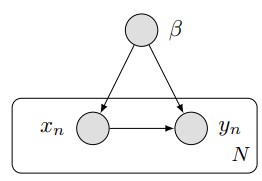
• $\beta=f_{\beta}\left(\epsilon_{\beta}\right), \quad \epsilon_{\beta} \sim s(\cdot)$
• $x_{n}=f_{x}\left(\epsilon_{x, n}, \beta\right) , \quad \epsilon_{x, n} \sim s(\cdot)$
• $y_{n}=f_{y}\left(\epsilon_{y, n}, x_{n}, \beta\right) \quad \epsilon_{y, n} \sim s(\cdot)$

이 셋팅에서, causal mechanism $f_y$에 관심있다. to calculate $p(y \mid \operatorname{do}(X=x), \beta)$

---

물론 Figure 1의 경우는 $p(y \mid \operatorname{do}(x), \beta)=p(y \mid x, \beta)$다.

즉, $\beta$를 관측하였다고 가정하면, $f_y$를 estimate할 수 있다. 예를 들어,

$$y_{n}=f\left(x_{n}, \beta \mid \theta\right)+\epsilon_{n}, \quad \epsilon \sim s(\cdot)$$ $$p(\theta \mid \mathbf{x}, \mathbf{y}, \beta) \propto p(\theta) p(\mathbf{y} \mid \mathbf{x}, \theta, \beta)$$

$\theta$를 VI나 MCMC로 구할 수 있다.

---

Deterministic 함수(linear, polynomial, …)를 쓰는 경우엔 hand-engineered low-order interactions를 사용하게 된다.

이러한 제한들을 완화하기 위해 Richer causal model을 세우는 방법을 소개하겠다.

2.2 Implicit Causal Models

IM은 structure에 대한 detail마저 unknown인 상황에서 generative process를 capture한다.

$$x=g(\epsilon \mid \theta), \quad \epsilon \sim s(\cdot)$$

이 때, $g$는 neural network로 둬서 nonlinear interaction을 다루게 된다.

이 역시도, randomness를 변수와 분리해서 input으로 넣기에 causal model의 structural invariance를 흉내낸다.

Causality를 강화하기 위해, ICM을 정의한다.

이 때, $g$는 structural equation이다.

Causal network가 Bayesian network를 확장했듯이 ICM은 IM을 확장한다.

3. ICMs with Latent Confounders

임의의 causal relation을 capture 할 수 있는 ICMs를 설명했다.

간결함을 위해, global structure는 주어졌다고 가정하겠다.

느낌상 Causal network까지만 known임을 가정하는 걸 말하는 것 같다.

3.1 Causal Inference with a Latent Confounder

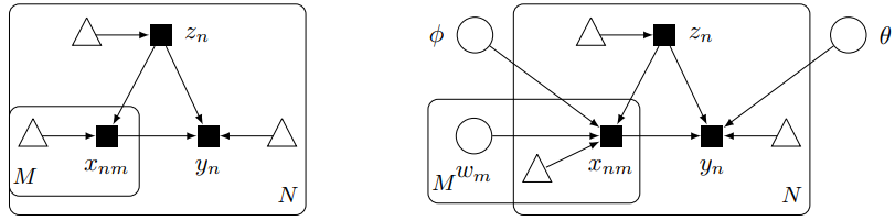
• $N$명의 개인들 (500~1만)
• $M$개의 SNP (10만~100만)
• $p\left(y \mid \operatorname{do}\left(x_{m}\right), x_{-m}\right)$에 관심있지만 $z_n$이 latent variable이라 unidentifiable이다.

왼쪽 그림은 causal graph로 세모는 noise를 나타낸다.

오른쪽 그림은 ICM으로 $\phi$와 $\theta$는 NN의 parameter로 mechanism에 대한 것이라 생각하자.

$z_n$은 population 관점에서 local latent variable이고

$w_m$은 SNP 관점에서 local latent variable이다.

Consider the ICM

$$\begin{aligned} z_{n} &=g_{z}\left(\epsilon_{z_{n}}\right), & & \epsilon_{z_{n}} \sim s(\cdot) \\ x_{n m} &=g_{x_{m}}\left(\epsilon_{x_{n m}}, z_{n} \mid w_{m}, \phi\right), & & \epsilon_{x_{n m}} \sim s(\cdot) \\ y_{n} &=g_{y}\left(\epsilon_{y_{n}}, x_{n, 1: M}, z_{n} \mid \theta\right), & & \epsilon_{y_{n}} \sim s(\cdot) \end{aligned}$$

$z_n$이 latent variable이므로 $f_y$의 posterior는 적분 꼴로 나온다.

$$p(\theta \mid \mathbf{x}, \mathbf{y})=\int p(\mathbf{z} \mid \mathbf{x}, \mathbf{y}) p(\theta \mid \mathbf{x}, \mathbf{y}, \mathbf{z}) \mathrm{d} \mathbf{z}$$

이 식을 해석하면, latent structure를 반영한 $p(\mathbf{z} \mid \mathbf{x}, \mathbf{y})$로 $p(\theta \mid \mathbf{x}, \mathbf{y}, \mathbf{z})$를 추론하게 된다.

Latent confounder를 갖고 causal inference를 하는 것은 위험할 수 있다.

$x$와 $y$를 갖고 $z$를 추정하고서, 추정된 $z$를 갖고서 mechanism을 추정하기에 bias를 가질 수 있다.

왜 이게 정당화될까?

Proposition 1

• True causal model이 ICM의 범위에 속한다고 가정하자.
• 그러면 $p(\theta \mid \mathbf{x}, \mathbf{y})$는 consistent estimator of causal mechanism $f_{y}$를 제공한다.

---

증명에 대한 직감으로는 $M$이 엄청 큰 상황에서 $p(z_n \mid x_{1:M})$은 $\delta_{z_{n}^{true}}$에 가까워진다.

같은 논리로 $N$이 커짐에 따라 true mechanism에 가까워지게 된다.

---

기존의 two-stage estimation 방법은 Astle & Balding $z$를 MAP로 대체한 것과 동일하다.

3.2 Implicit Causal Model with a Latent Confounder

• $z_n$

  • $g_z$는 그저 identity function으로 두고
  • Prior는 standard normal로 두고
  • 차원 $K$는 적당히 큰 정도로 설정한다. (hyperparameter)

• $x_{nm}$

  • GWAS에서 성공한 factor analysis formulation에 기반을 한다.

  • $0$은 two major alleles, 1은 one major allele, 그리고 2는 two minor alleles를 의미한다.

  • $x_{nm} | z_n, w_m \sim \operatorname B(2, \pi_{nm})$ where $\operatorname{logit} \pi_{n m}=z_{n}^{\top} w_{m}$

  • $w_m$의 prior는 비교모델인 logistic factor analysis처럼 standard normal로 둔다.

  • 그 경우에, $w_m$은 principal component의 역할로 $M$차원의 원본을 $K$차원의 embedding이 된다.

  • Logit을 NN으로 둬서 좀 더 완화된 가정을 둬도 된다. $\operatorname{logit} \pi_{n m}=\mathrm{NN}\left(\left[z_{n}, w_{m}\right] \mid \phi\right)$

• $y_n$

  • $y_{n}=\left[x_{n, 1: M}, z_{n}\right]^{\top} \theta+\epsilon_{n}, \quad \epsilon_{n} \sim \operatorname{Normal}(0,1)$

  • $y_{n}=\mathrm{NN}\left(\left[x_{n, 1: M}, z_{n}, \epsilon\right] \mid \theta\right), \quad \epsilon_{n} \sim \operatorname{Normal}(0,1)$

  • SNP에서 hidden layer로 가는 부분에 group Lasso prior를 둬서 sparse input 만으로 $y_n$을 예측하도록 유도하자.

    Group Lasso prior도 한번 봐야겠다.

  • 나머지는 standard normal prior를 사용하자.

4. Likelihood-Free Variational Inference

Given GWAS data, we want to infer $p(\theta \mid \mathbf x, \mathbf y)$.

이는 joint posterior를 추론한 뒤에 marginalize를 하거나, 중간 과정을 collapse하면 된다.

$$p\left(z_{1: N}, w_{1: M}, \phi, \theta \mid \mathbf{x}, \mathbf{y}\right) \propto p(\phi) p(\theta) \prod_{n=1}^{N}\left[p\left(z_{n}\right) p\left(y_{n} \mid x_{n, 1: M}, z_{n}, \theta\right) \prod_{m=1}^{M} p\left(w_{m}\right) p\left(x_{n m} \mid z_{n}, w_{m}, \phi\right)\right]$$

다만 어려움은 $p\left(y_{n} \mid x_{n, 1: M}, z_{n}, \theta\right), p\left(x_{n m} \mid z_{n}, w_{m}, \phi\right)$를 모른다는 것이다.

이 경우, LFVI를 적용하면 된다.

VI과정에서,

• $q\left(w_{m}\right)=\operatorname{Normal}\left(w_{m} ; \mu_{w_{m}}, \sigma_{w_{m}} I\right)$
• $q\left(z_{n}\right)=\operatorname{Normal}\left(z_{n} ; \mu_{z_{n}}, \sigma_{z_{n}} I\right)$
• $q(\theta) = \delta_{\theta}$
• $q(\phi) = \delta_{\phi}$