0. Abstract

SCM은 mechanism과 exogeneous sources of random variation을 나타낸다.

NN은 universal approximability의 특징을 갖는다.

아마 SCM의 함수를 NN으로 대체하여 학습할 수 있다는 생각을 해봤을 수 있다.

이 논문에선

expressivity와 learnability의 개념을 구분지어서 안되는 것을 보인다.
무엇이 데이터로부터 학습될 수 있는 지에 대한 causal hierarchy theorem(CHT)이 neural causal model(NCM)에 적용될 수 있음을 보인다.

예를 들어, 단순한 임의의 complex and expressive NN은 observational data만 갖고서 interventional effect를 예측할 수 없다.

이 결과를 갖고서,

NCM이라는 특수한 종류의 SCM을 도입하고
causal inference를 수행하기 위해 필요한 structural constraints를 위한 inductive bias를 formalize한다.

NCM이라는 새로운 model class로 causal identification and estimation task에 집중한다.

1. Introduction

Universality가 말하길 neural model은 임의의 precision을 갖는 아무 함수를 approximate할 수 있다.

이 특징은 대부분의 task가 함수로 모델링 될 수 있기에, 올바른 조건 하에서 NN은 어렵고 흥미로운 AI task를 해결할 수 있다고 믿게 만든다.

이 믿음은 게임, 음성인식, 컴퓨터비전 등 에서 실용적인 성공에 의해 확증되어간다.

이 논문에선, NN의 universality를 causal reasoning의 영역에서 조사해보겠다.

Causal-neural connection을 이해하기 위해, 두가지 개념이 중요하다.

SCM
Pearl Causal Hierarchy (PCH) : fully specified SCM induces a collection of distribution

PCH의 중요성은 인간의 활동으로 연관지어질 수 있는 cognitive capability를 formal하게 구분짓기 때문이다.

“seeing” : layer 1
“doing” : layer 2 : the effects of interventions
“imagining” : layer 3 : the counterfactuals

각 layer들은

구분된 formal language로 표현될 수 있고
inference의 종류들을 구분하는데 도움되는 query를 나타낸다.

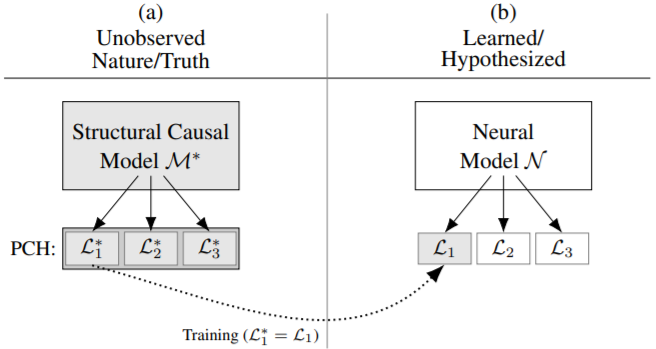
Fig. 1(a) 해석

SCM $M^\star$는 PCH의 layer들 $L_{1}^{\star}, L_{2}^{\star}, L_{3}^{\star}$을 induce한다.
Challenging inferential task는 $M^\star$의 일부 관측으로 PCH의 특정 layer를 recover하려고 할 때 발생한다.
구체적으로, intervention($L_2^\star$) effect에 대한 statement가 필요할 때, $L_1^\star$의 데이터만 passive하게 수집된 상황이 있다.

Fig. 1(b) 해석

$M^*$로 생성된 data를 사용해 neural model을 학습해보려 할 수 있다.
일반적인 consistency를 위해선 $N$은 $M^\star$의 generating distribution을 따라할 만큼 capable해야 한다.
Universality of neural model 하에서, 이는 large sample에서 만족될 것이다.
Question : 학습된 모델이 $M^\star$에 의해 생성된 $L_2$ distribution과 일치하는 intervention effect를 예측하는 능력이 있는 proxy로서 작동할 수 있을까?
Answer : Corollary1에서 일반적으로 확인될 수 없음이라고 하나, 직감적으로 말하면 $L_1 = L_1^\star$이지만 $L_2 \neq L_2^\star$인 여러 neural model이 있기 때문이다.

즉, neural model이 $M^*$를 표현할만한 능력이 있더라도, consistency w.r.t. $L_1$이 higher-layer inferences를 보장하는 데는 불충분 조건이다.

이에 대한 직감으로는 $L_1$이 똑같은데 $L_2$가 다른 neural model이 너무 많기 때문이다.

이는 causal inference 분야에서 CE identification과 estimation task에 속한다.

Identification
- do-calculus에 기반해 많이 연구됐다.
- $M^*$에 대한 causal diagram 또는 markov equivalence Causal identification under Markov equivalence 하에서,
- causal query가 $P(v)$로 unique하게 결정되는 지 확인한다.
- 이 task를 해결하는 neural method는 없다.
Estimation
- Identifiable이라고 결정됐을 때 시작하는 task이다.
- 딥러닝 테크닉이 실용적인 performance로 effect를 estimate하는 연구들은 굉장히 많이 있다.
- Backdoor criterion (conditional ignorability) : 60, 49, 45, 30, 65, 66, 34, 61, 15, 25
- O.W. (frontdoor, napkin) : 31, 32, 33
- 이들은 target interventional distribution에 대응하는 특정 estimand를 최적화하는 방식이다.

여전히 임의의 셋팅에서 $M^*$에 대한 proxy로서 NN을 generative model로서 causal identification+estimation task를 어떻게 수행할 지는 잘 알려지지 않았다.

real world(high dimensional domain)로 확장 가능하고, tranditional symbolic approach처럼 inference의 유효성을 보존하는 causal-neural framework를 개발하는 것이 목표이다.

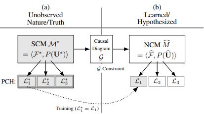
기존에 identifiability를 위해 causal diagram이 do-calculus에 필요한 assumption을 나타냈듯이, neural causal model(NCM)은

gradient descent로 적용가능하고
통합적인 방식으로 두 task를 수행하게하는

invariances를 inductive bias로서 encode한다.

Contributions

2장에서 GD가 가능한 SCM의 특수 타입인 NCM을 소개하고, 이의 properties를 증명한다.
- universal expresiveness
- certain structural invariance를 나타내는 inductive bias를 encode하는 능력
- expressivity에도 불구하고, CHT를 준수한다.
3장
- Neural identification problem을 formalize하고 (Def. 8)
- causal diagram과 NCM 사이의 duality를 증명하고 (Thm. 4)
- NCM에서 inference를 수행하는 방법을 소개하고 (Corol. 2-3)
- NCM의 학습과 effect identifiability를 동시에 결정하는 알고리즘을 소개한다. (Alg. 1, Corol. 4)
4장
- 이러한 결과들에 기반해 GD로 CE를 identify하면서 estimate하는 알고리즘을 개발한다. (Alg. 2)

1.1 Preliminaries

Definition 1 (SCM)

An SCM is a 4-tuple $\langle\mathbf{U}, \mathbf{V}, \mathcal{F}, P(\mathbf{U})\rangle$ where

$\mathbf U$ is a set of exogenous variables
$\mathbf V = \left\{V_{1}, V_{2}, \ldots, V_{n}\right\}$ is a set endogenous variables
$\mathcal F = \left\{f_{V_{1}}, f_{V_{2}}, \ldots, f_{V_{n}}\right\}$ is a set of functions s.t. $v_i = f_{V_{i}}\left(\mathbf{pa}_{V_{i}}, \mathbf{u}_{V_{i}}\right)$
$P(\mathbf{u})$ is a probability function defined over the domain of $\mathbf U$

각 SCM $\mathcal M$은 causal diagram $G$를 induce한다.

변수들간의 관계는 $\left(V_{j} \rightarrow V_{i}\right)$와 $V_{j} \leftrightarrow V_{i}$로 이뤄진다.

전자는 $V_j$가 $\mathbf{Pa}_{V_i}$에 속하는 경우이고, 후자는 $\mathbf{U}_{V_{i}} \cap \mathbf{U}_{V_{j}} = \not \emptyset$인 경우이다.

Definition 2 (Layers 1, 2 Valuations)

An SCM $\mathcal M$ induces layer $L_2(\mathcal M)$ a set of interventional distributions over $\mathbf V$.

For each $\mathbf{Y} \subseteq \mathbf{V}$,

$P^{\mathcal{M}}\left(\mathbf{y}_{\mathbf{x}}\right)=\sum_{\left\{\mathbf{u} \mid \mathbf{Y}_{\mathbf{x}}(\mathbf{u})=\mathbf{y}\right\}} P(\mathbf{u})$

When fixed $\mathbf X = \emptyset$, it is defined as $L_1(\mathcal M)$

2. Neural Causal Models and the Causal Hierarchy Theorem

이 섹션에서, expressiveness와 learnability 사이의 tension(?)을 푸는 데(?)에 집중한다.

이를 위해 SCM의 special class로서,

Optimization을 허용하는 NN에 기반해
Unobserved true SCM $\mathcal M^\star$에 대한 proxy로 작동할 잠재력이 있는

Definition 3 (NCM)

NCM $\widehat{M}(\boldsymbol{\theta})$ over variables $\mathbf V$ with parameters $\boldsymbol{\theta}=\left\{\theta_{V_{i}}: V_{i} \in \mathbf{V}\right\}$ is an SCM $\langle\widehat{\mathbf{U}}, \mathbf{V}, \widehat{\mathcal{F}}, \widehat{P}(\widehat{\mathbf{U}})\rangle$ s.t.

$\widehat{\mathbf{U}} \subseteq\left\{\widehat{U}_{\mathbf{C}}: \mathbf{C} \subseteq \mathbf{V}\right\}$
- $\widehat{U}_{\mathbf C}$ is associated with $\mathbf C$
- $\mathcal D _{\widehat U_{\mathbf C}} = \left[ 0, 1\right]$
$\widehat{\mathcal{F}}=\left\{\hat{f}_{V_{i}}: V_{i} \in \mathbf{V}\right\}$
- $\hat f_{V_i}$ is a feedforward NN parameterized by $\theta_{V_i} \in \boldsymbol \theta$
- $V_i = \hat f_{V_i}(\mathbf{U}_{V_{i}} \cup \mathbf{P a}_{V_{i}})$
- $\mathbf{U}_{V_{i}}=\left\{\widehat{U}_{\mathbf{C}} \in \widehat{\mathbf{U}}: V_{i} \in \mathbf{C}\right\}$
$\widehat{P}(\widehat{U}_{\mathbf C}) = \operatorname{Unif}(0,1)$

Remark

NCM은 SCM이므로, PCH layers와 관련된 distribution을 생성할 능력이 있다.
NCM $\in$ SCM

NCM과 SCM의 expressiveness를 비교하기 위해, consistency 개념을 formalize하겠다.

Definition 4 ($P^{(L_i)}$-Consistency)

Consider two SCMs $\mathcal M_1$ and $\mathcal M_2$.

$\mathcal M_2$ is said to be $P^{(L_i)}$-consistent w.r.t. $\mathcal M_1$ if $L_{i}\left(\mathcal{M}_{1}\right)=L_{i}\left(\mathcal{M}_{2}\right)$

위의 정의는 NCM뿐만 아니라 일반적인 SCM에도 적용된다.

\\mbaetghiNCM은 true SCM $\mathcal M^*$의 함수들과 (observational / interventional / counterfactual) distribution을 완벽하게 표현할 수 있다.

Theorem 1 (NCM Expressiveness)

$^ \forall$SCM $\mathcal M^\star = \langle\mathbf{U}, \mathbf{V}, \mathcal{F}, P(\mathbf{U})\rangle$, $^{\exists}$NCM $\widehat{M}(\boldsymbol{\theta})=\langle\widehat{\mathbf{U}}, \mathbf{V}, \widehat{\mathcal{F}}, \widehat{P}(\widehat{\mathbf{U}})\rangle$ s.t.

$\widehat{M} \text { is } L_{3} \text {-consistent w.r.t. } \mathcal{M}$

자연스러운 질문은 observational data로 학습해서 $\mathcal M^\star$의 proxy로 NCM을 사용해 inference를 수행할 수 있을 지에 대한 여부이다.

불행히도, 보통 안된다.

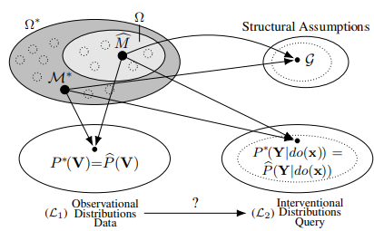
Corollary 1 (Neural Causal Hierarchy Theorem (N-CHT)).

Let $\Omega^\star$ and $\Omega$ be the sets of all SCMs and NCMs.

$\text{Layer $j$ of the causal hierarchy for NCMs collapses to Layer $i(<j)$ relative to $M^\star \in Ω^\star$}$

if $L_{i}\left(\mathcal{M}^{\star}\right)=L_{i}(\widehat{M})$ implies $L_{j}\left(\mathcal{M}^{\star}\right)=L_{j}(\widehat{M})$ for all $\widehat{M} \in \Omega$.

With respect to lebesgue measure over SCMs, the subset in which Layer $j$ of NCMs collapses to Layer $i$ has measure zero.

Corollary 1은 NCM $\widehat {\mathcal M}$이 expressive 측면에서 SCM $\mathcal M ^{\star}$의 적합한 대체제 일지라도, PCH layers 사이의 inference가 어려다는 것을 나타낸다.

2.1 A Family of Neural-Interventional Constraints (Inductive Bias)

Constraints about $\mathcal M^{\star}$를 알아보자.

이는 hypothesis space를 좁히고 valid cross-layer inference를 허용하게 해줄 수도 있다.

SCM은 interventional distribution $\mathcal P$와 causal diagram $\mathcal G$로 이루어져 있다.

$\mathcal G$는 $\mathcal P$상에 constraint를 주고 이는 cross-layer inference를 수행하는데 유용하다.

간결함을 위해, observational data로부터 interventional inference을 수행하는 것에 집중한다.

Definition 5 ($\mathcal G$ -Consistency)

Let $\mathcal G$ be the causal diagram induced by SCM $\mathcal M^\star$.

$\text{For any SCM $\mathcal M$, $\mathcal M$ is $\mathcal G$-consistent w.r.t. $\mathcal M^{\star}$}$

, if $\mathcal G$ is a CBN for $L_2(\mathcal M)$

$\mathcal M^\star$처럼 $\mathcal P$상에 constraint를 부과해야 한다.

Definition 6 ($C^2$-Component)

A subset $\mathbf C \subseteq \mathbf V$ is complete confounded component($C^2$-Component) if

$^{\forall}V_{i}, V_{i} \in \mathbf{C}$, $V_i \leftrightarrow V_j$
$\mathbf C$ is maximal

Definition 7 ($\mathcal G$-Constrained NCM)

Let $G$ be the causal diagram induced by SCM $\mathcal M^\star$.

Construct NCM $\widehat M$ as follows

Choose $\widehat {\mathbf U}$ so that $\widehat{U}_{\mathbf{C}} \in \widehat{\mathbf{U}}$ iff $\mathbf C$ is a $C^2$-component.
For each $V_i \in \mathbf V$, choose $\mathbf{P a}_{V_{i}} \subseteq \mathbf{V}$ s.t. $V_j \in \mathbf {Pa}_{V_i}$ implies $V_j \rightarrow V_i$ in $\mathcal G$

Theorem 2 (NCM $\mathcal G$-Consistency)

Any $\mathcal G$-constrained NCM $\widehat M(\boldsymbol \theta)$ is $\mathcal G$-consistent.

Theorem 3 ($L_2- \mathcal G$ Representation)

$^{\forall} \text{SCM }\mathcal M^{\star}$ that induces causal diagram $\mathcal G$,

$^{\exists}\mathcal G$-constrained NCM $\widehat M(\boldsymbol \theta) = \langle\widehat{\mathbf{U}}, \mathbf{V}, \widehat{\mathcal{F}}, \widehat{P}(\widehat{\mathbf{U}})\rangle$ that $L_2$-consistent w.r.t. $\mathcal M^\star$.

NCM에 constraint를 부과함에도, 여전히 $\mathcal M^\star$의 Layer2를 나타낼만큼 expressive하다.

이 constraint를 inductive bais로 활용하면, $\widehat{\mathcal M}$은 특정 조건 하에서, $L_2$ consistency를 만족할 수 있다.

3. The Neural Identification Problem

$\mathcal G$-constarined NCM에서 causal inference가 가능한 지를 조사해보자.

Definition 8 (Neural Effect Identification)

Let $\Omega^\star$ be the set of all SCMs, and $\Omega (\mathcal G)$ the set of $\mathcal G$-constrained NCMs.

The CE $P(\mathbf{y} \mid d o(\mathbf{x}))$ is said to be neural identifiable from $\Omega(\mathcal G)$ and observational data

iff

$P^{\mathcal{M}^{\star}}(\mathbf{y} \mid d o(\mathbf{x}))=P^{\widehat{M}}(\mathbf{y} \mid d o(\mathbf{x}))$ for every $(\mathcal M^\star, \widehat{\mathcal M}) \in \Omega^\star \times \Omega(\mathcal G)$ s.t.

$\mathcal M^\star$ induces $\mathcal G$
$P(\mathbf v) = P^{\mathcal M^\star}(\mathbf v) = P^{\widehat{\mathcal M}}(\mathbf v)$

Theorem 4 (Graphical-Neural Equivalence (Dual ID)).

Let $\Omega ^{\star}$ be the set of all SCMs and $\Omega$ th eset of NCMs.

Consider the true SCM $\mathcal M^\star$ and the corresponding causal diagram $\mathcal G$.

Let $Q = P(\mathbf y \mid do(\mathbf x))$ be the query of interest and $P(\mathbf v)$ be the observational distribution.

Then, $Q$ is neural identifiable from $\Omega(\mathcal G)$ and $P(\mathbf v)$ iff $Q$ is identifiable from $\mathcal G$ and $P(\mathbf v)$

Theorem 4는 identification이 유지됨을 의미한다.

NCM을 통해 inference까지 하는 것이 목표이기 때문에, theorem 4는 이게 가능함을 보장해준다.

Corollary 2 (Neural Mutilation (Operational ID))

Consider

the true SCM $\mathcal M^\star \in \Omega ^\star$
causal diagram $\mathcal G$
observational distribution $P(\mathbf v)$
target query $Q = P^{\mathcal M^\star}(\mathbf y \mid do(\mathbf x))$

Let $\widehat {\mathcal M} \in \Omega (\mathcal G)$ be a $\mathcal G$-constrained NCM that is $L_1$-consistent with $\mathcal M^\star$.

If $Q$ is identifiable from $\mathcal G$ and $P(\mathbf v)$, then $Q$ is computable through a multilation process on $\widehat{\mathcal M}$

$L_1$-consistency
$\mathcal G$-constraint
identifiable

일 경우에, NCM에 절단과정으로 inference가 수행될 수 있음을 나타낸다.

Markovian SCM은 $U_i$가 한개의 $V_i$에만 영향을 주는 구조이고, interventional distribution이 identifiable하다.

Corollary 3 (Markovian Identification)

Whenever the $\mathcal G$-constrained NCM $\widetilde {\mathcal M}$ is Markovian, $P(\mathbf y \mid do(\mathbf x))$ is always identifiable via the proxy NCM.

Non-Markovian case에 대해선 알고리즘1이 특정 effect가 observational data로 부터 identifiable한 지를 결정한다.

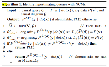
놀랍게도, 이 procedure는 necessary and sufficient 하다는 것이다.

이는 딥러닝이 identifiability를 결정하는 데에 do-calculus처럼 강력함을 의미한다.

Corollary 4 (Soundness and Completeness)

Let $\Omega^\star$ be the set of all SCMs.

Let $\mathcal M^\star \in \Omega^\star$ be the true SCM inducing causal diagram $\mathcal G$.

Let $Q = P(\mathbf y \mid do(\mathbf x))$ be a query of interest.

Let $\widehat Q$ be the result from running Algorithm 1 w/ inputs

$P^{}(\mathbf{v})=L_{1}\left(\mathcal{M}^{}\right)>0$
$\mathcal G$
$Q$

Then, $Q$ is identifiable iff $\widehat Q$ is not FAIL.

Moreover, if $\widehat Q$ is not FAIL, then $P^{\mathcal{M}^{*}}(\mathbf{y} \mid d o(\mathbf{x}))$.

4. The Neural Estimation Problem

Identifiability가 asymptotic theory에 의해 해결됐으나, finite sample 하에서 estimating CE를 고려해보자.

간결함을 위해, 모든 $V_i$는 binary를 가정하겠으나, continuous variable로 확장될 수 있는 논의를 하겠다.

Gumbel-Max trick에 기반해서, NCM을 정의하자.

$\begin{cases}\mathbf{V} & := \mathbf V \\ \widehat{\mathbf{U}}&:=\left\{U_{\mathbf{C}}: \mathbf{C} \in C^{2}(\mathcal{G})\right\} \cup\left\{G_{V_{i}}: V_{i} \in \mathbf{V}\right\} \\ \widehat{\mathcal{F}} & := \left\{f_{V_{i}}:=\arg \max _{j \in\{0,1\}} \left [ g_{j, V_{i}}+\left\{\begin{array}{ll} \log \sigma\left(\phi_{V_{i}}\left(\mathbf{p a}_{V_{i}}, \mathbf{u}_{V_{i}}^{c} ; \theta_{V_{i}}\right)\right) & j=1 \\ \log \left(1-\sigma\left(\phi_{V_{i}}\left(\mathbf{p a}_{V_{i}}, \mathbf{u}_{V_{i}}^{c} ; \theta_{V_{i}}\right)\right)\right) & j=0 \end{array}\right.\right. \right] \\ P(\widehat{\mathbf{U}}) & := \left\{U_{\mathbf{C}} \sim \operatorname{Unif}(0,1): U_{\mathbf{C}} \in \mathbf{U}\right\} \cup \left\{G_{j, V_{i}} \sim \operatorname{Gumbel}(0,1): V_{i} \in \mathbf{V}, j \in\{0,1\}\right\} \end{cases}$ $\begin{aligned} P^{\widehat{M}(\mathcal{G} ; \boldsymbol{\theta})}(\mathbf{v} \mid d o(\mathbf{x})) &= \sum_{\widehat{\mathbf u}}\prod_{V_i \in \mathbf V \setminus \mathbf X}P(V_i = v_i \mid \mathbf u_{V_i}) P(\widehat{\mathbf u}) \\ &= \sum_{\widehat{\mathbf u}}\prod_{V_i \in \mathbf V \setminus \mathbf X}\tilde{\sigma}_{v_{i}} P(\widehat{\mathbf u}) \quad \text{where $\tilde{\sigma}_{v_{i}}:= \begin{cases}\sigma\left(\phi_{i}\left(\mathbf{p} \mathbf{a}_{V_{i}}, \mathbf{u}_{V_{i}}^{c} ; \theta_{V_{i}}\right)\right) & v_{i}=1 \\ 1-\sigma\left(\phi_{i}\left(\mathbf{p a}_{V_{i}}, \mathbf{u}_{V_{i}}^{c} ; \theta_{V_{i}}\right)\right) & v_{i}=0\end{cases}$} \\ &\approx \frac{1}{m} \sum_{j=1}^{m} \prod_{V_{i} \in \mathbf{V} \backslash \mathbf{X}} \tilde{\sigma}_{v_{i}} \quad \text{where $\left\{\mathbf{u}_{j}^{c}\right\}_{j=1}^{m} \sim P\left(\mathbf{U}^{c}\right)$} \quad \because \tilde{\sigma}_{v_{i}} \text{ is indep to $g_{V_i}$} \end{aligned}$

Algorithm 1의 line 2~3은 $L_1$consistency를 요구한다.

하지만 finite sample만 있기 때문에, data의 likelihood를 최대화하여 NCM을 estimate해야한다.

추가로 CE를 최대화(혹은 최소화)하기 위해, additional term을 추가하여,

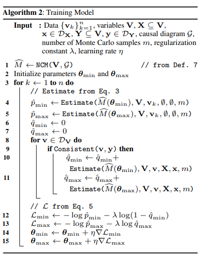
$\frac{1}{n} \sum_{k=1}^{n}-\log \widehat{P}_{m}^{\widehat{M}}\left(\mathbf{v}_{k}\right)-\lambda \log \widehat{P}_{m}^{\widehat{M}}(\mathbf{y} \mid d o(\mathbf{x}))$

실제론, identifiability test는 hypothesis testing에 의존하게 된다.

$\left|f\left(\widehat{M}\left(\boldsymbol{\theta}_{\max }\right)\right)-f\left(\widehat{M}\left(\boldsymbol{\theta}_{\min }\right)\right)\right|<\tau$

5. Experiments

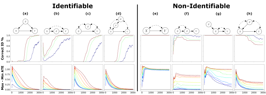
8개의 SCM에 대해서
$\tau=0.01, 0.03, 0.05$ (파랑, 초록, 빨강) 별로 identifiability classification accuracy이고
1~99 percentile of max-min gap이다.

Study Repo

The Causal-Neural Connection Expressiveness, Learnability, and Inference