0. Abstract

X-learner는 CATE의 structural property를 활용하기에
- T-learner (GCOM) 과 비교하여
- treatment group imbalance 상황에서 유용
CATE function이 linear고 Response function이 Lipshitz continuous면
- 수렴보장

1. Introduction

개인별, context 별로 TE가 차이가 날 지
즉, CATE를 알아내는 문제에 X-learner라는 프레임워크를 도입
이는 CATE estimation 문제를 두개의 sub regression problem으로 나눔
- base learner로 Conditional Expectation을 학습
  - RF, BART, NN
- 실제 outcome들과의 차이를 분석

만약 ITE를 관측할 수 있다면,
- covariate => ITE
- 함수를 학습해서 CATE function을 추론할 수 있다.
ITE를 알 일은 없지만,
- X-learner는 observed ITE을 ITE estimate에 써먹고
- 추정된 ITE를 estimate하는 CATE function을 학습한다.

Notation

$(Y_i(0), Y_i(1), X_i, W_i) \sim \mathcal P$
- $X_i \in \mathbb R^d$ : covariate
- $W_i \in \{ 0, 1 \}$ : treatment assignment
- $i \in [N]$
$D_i := Y_i(1) - Y_i(0)$
$\mu_0(x) := \mathbb E [Y(0) \mid X=x]$
$\mu_1(x) := \mathbb E [Y(1) \mid X= x]$
$\tau(x) := \mu_1(x) - \mu_0(x)$
$\mathcal D = (Y_i, X_i, W_i)_{1\leq i \leq N}$ : observed data
$n := \sum_i W_i$ ; the number of obs in treatment group
$m := N-n$
$\text{EMSE} (\mathcal P , \hat \tau) = \mathbb E [(\tau(\mathcal X) - \hat \tau(\mathcal X))^2]$
- Expected Mean Squared Error for estimating CATE

$\mathcal P$ generates

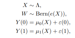
Assumption

T-learner
- $\mu_0(x) = \mathbb E [Y(0) \mid X=x]$를 $\{(X_i, Y_i)\}_{W_i = 0}$ 로 학습
- $\mu_1(x) = \mathbb E [Y(1) \mid X=x]$를 $\{(X_i, Y_i)\}_{W_i = 1}$ 로 학습
- $\hat \tau_T(x) = \hat \mu_1(x) - \hat \mu_0(x)$
S-learner
- $\mu(x, w) := \mathbb E[Y^{obs} \mid X=x, W=w]$ 를 $\{(X_i, W_i, Y_i)\}$ 로 학습
- $\hat \tau_S(x) = \hat \mu(x, 1) - \hat \mu(x, 0)$
X-learner
- $\mu_0(x) = \mathbb E [Y(0) \mid X=x]$를 $\{(X_i, Y_i)\}_{W_i = 0}$ 로 학습
- $\mu_1(x) = \mathbb E [Y(1) \mid X=x]$를 $\{(X_i, Y_i)\}_{W_i = 1}$ 로 학습
- Impute
  - $\tilde D_i^1 := Y_i^1 - \hat \mu_0(X_i^1)$ for $i : W_i=1$
  - $\tilde D_i^0 := \hat \mu_1(X_i^0) - Y_i^0$ for $i : W_i=0$
- $\tau_1(x) = \mathbb E [\tilde D ^1 \mid X = x]$를 $\{(X_i^1, \tilde D_i^1)\}$ 로 학습
- $\tau_0(x) = \mathbb E [\tilde D ^0 \mid X = x]$를 $\{(X_i^0, \tilde D_i^0)\}$ 로 학습
- $\hat \tau(x) = g(x) \hat \tau_0(x) + (1-g(x))\hat\tau_1(x)$

$Y_i^1 = \mu_1(x) + \epsilon(0)$
$Y_i^0 = \mu_0(x) + \epsilon(0)$
$\hat \mu_0(x) = \mu_0(x)$ and $\hat \mu_1(x) = \mu_1(x)$ implies
- $\tau(x) = \mathbb E[\tilde D^1 \mid X=x] = \mathbb E[\tilde D^0 \mid X=x]$
즉, 둘 다 학습하고 합치는 게 타당하다.
실험상 적은 샘플에 더 가중치를 주는 propensity score가 $g(x)$로 어울렸음.
$\hat \tau_0$과 $\hat \tau_1$에 대한 분산추정이 가능하면 분산을 최소화하는 $g(x)$도 좋음

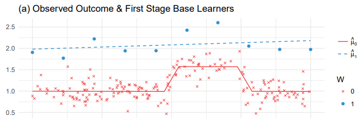
CATE가 constant 1인 경우이다.
$\mu_1(x) := \mathbb E [Y(1) \mid X= x]$
- 학습하는 데에 샘플이 적기에 오버피팅 문제가 있으니
- sample이 10개라 단순선형회귀모형를 채택
$\mu_0(x) := \mathbb E [Y(0) \mid X= x]$
- $x \in [0, 0.5]$에서 outcome이 다름
- 샘플이 충분하기 때문에 piecewise linear model을 사용
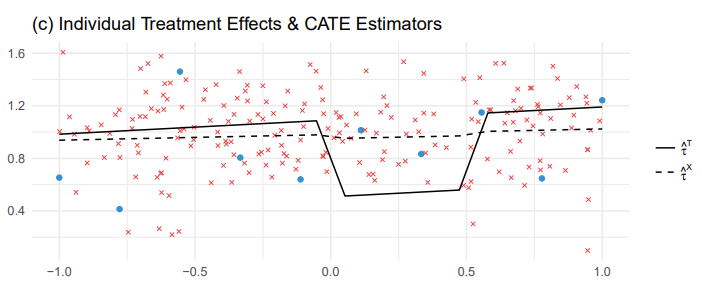
T-learner는 단순하게 $\hat \tau_T(x) = \hat \mu_1(x) - \hat \mu_0(x)$ 채택
- 비록 $\tau(x)$는 단순한 상수지만 복잡한 함수가 되어버림
- 각 estimator는 오버피팅을 피했으나 결과가 unreasonable함
서로를 고려하면서 학습하는 구조로 가야함
- X-learner는 structural information을 활용
- 특히, imbalance design에서 유용
비록 첫 시작은 똑같이 $\hat \mu_1(x),\hat \mu_0(x)$ 를 학습하지만,
- $\hat \tau_1$ 학습에 $\hat \mu_0$을 활용
- $\hat \tau_0(x)$ 학습에 $\hat \mu_1$을 활용
- 이게 X-learner라고 부르는 이유